Getting started
STREAM is a Windows desktop application for digital elevation models (DEM), orthophotos, point clouds and CAD drawings. The typical flow is always the same: load data → draw, measure and analyse → export.
The STREAM window
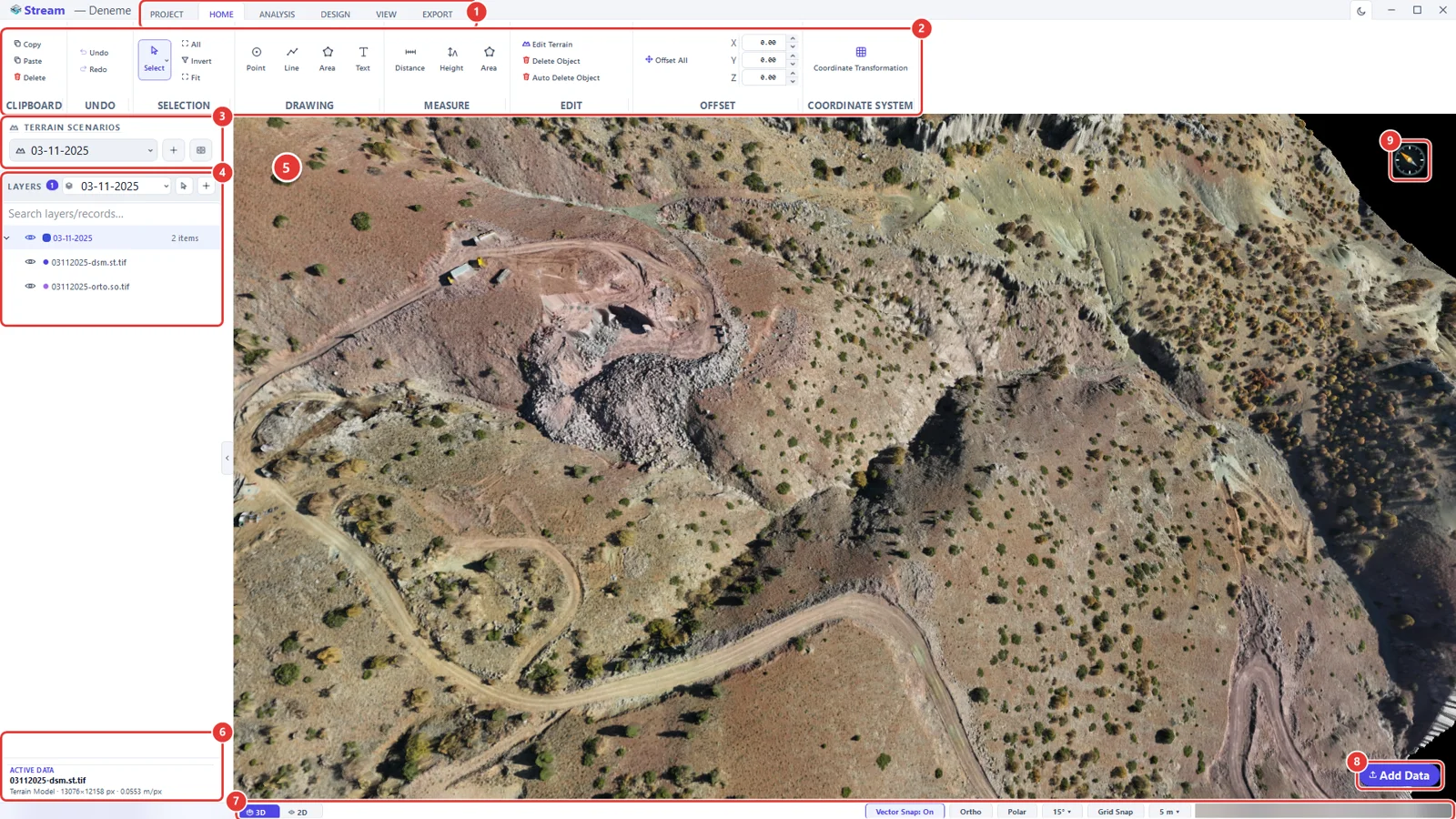
- Ribbon tabs — PROJECT, HOME, ANALYSIS, DESIGN, VIEW and EXPORT. When you select an object or start an analysis, a context tab for it (for example AREA, LINE or SLOPE) appears at the end of the row.
- Ribbon — the tools of the active tab, grouped under a title (DRAWING, MEASURE, EDIT …).
- TERRAIN SCENARIOS — the surveys of the same site kept side by side; the list switches between them.
- LAYERS — every dataset, drawing and analysis result of the active scenario, with an eye icon to show or hide each one.
- 3D view — the terrain itself. This is where you navigate, draw and click.
- ACTIVE DATA — live numbers for whatever is selected or being measured: lengths, areas, volumes.
- Status bar — the 3D / 2D switch, the snapping switches (Vector Snap, Ortho, Polar, Grid Snap), the project coordinate system on the left and the cursor coordinates on the right.
- Add Data — loads terrain, imagery, point clouds and CAD files into the project.
- Compass — shows where north is; double-click it for a north-up, top-down view.
The Home Screen
When STREAM starts, the Home Screen is the first thing you see. Click the Stream brand at the top-left of the window to bring it back at any time.
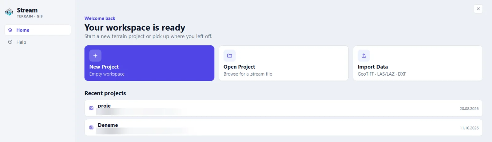
- Choose one of the three cards: New Project (an empty workspace), Open Project (browse for a saved project file) or Import Data (GeoTIFF, LAS/LAZ, DXF and more — several files can be picked at once).
- Or click a row under Recent projects to continue where you left off.
- Help, Settings and About on the left are pages of this same screen, not separate windows.
- Back to workspace at the top-right returns to the map. Esc does the same.
Opening and saving a project
The PROJECT tab manages project files.

- New starts an empty project. Open opens a saved one; the arrow on the button lists the recent projects.
- Save writes all layers, drawings, measurements and terrain scenarios into one project file. Save As writes a copy under a new name.
- Close closes the project and returns to the Home Screen.
- Shortcuts: Ctrl+N new · Ctrl+O open · Ctrl+S save · Ctrl+Shift+S save as.
Adding data
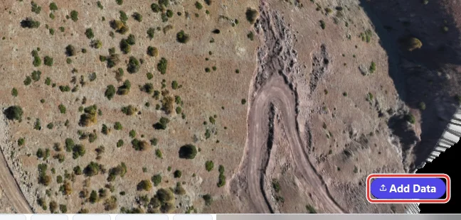
- Click Add Data at the bottom-right corner of the view (shortcut L).
- Pick one or more files. STREAM reads:
- DEM (GeoTIFF) — elevation data; this builds the 3D terrain.
- Orthophoto (GeoTIFF) — an aerial image draped over the terrain.
- Point cloud (LAS / LAZ) — you choose whether a DEM is built from the ground points or from all points, and whether an orthophoto is made from the point colours.
- CAD drawing (DXF), LandXML, SHP / GeoJSON / GPKG — vectors become editable points, lines and areas.
- Each file is prepared in a card at the bottom-right of the view. When the card says the data is ready, press Add to put it into the project, or Cancel to discard it.
- The new dataset appears as a row in LAYERS.
Moving around the terrain
When no tool is active, the mouse navigates the map and selects objects.
Mouse and keyboard
| Action | What it does |
|---|---|
| Left-button drag | Pans the map |
| Mouse wheel | Zooms toward or away from the point under the cursor |
| Middle-button drag (press the wheel) | Orbits the camera in 3D mode |
| Arrow keys | Pan · Shift + arrow rotates and tilts in 3D mode |
| + / − | Zoom in / out |
| Double-click the compass | Top-down view with north up |
| Ctrl+Z / Ctrl+Y | Undo / redo |
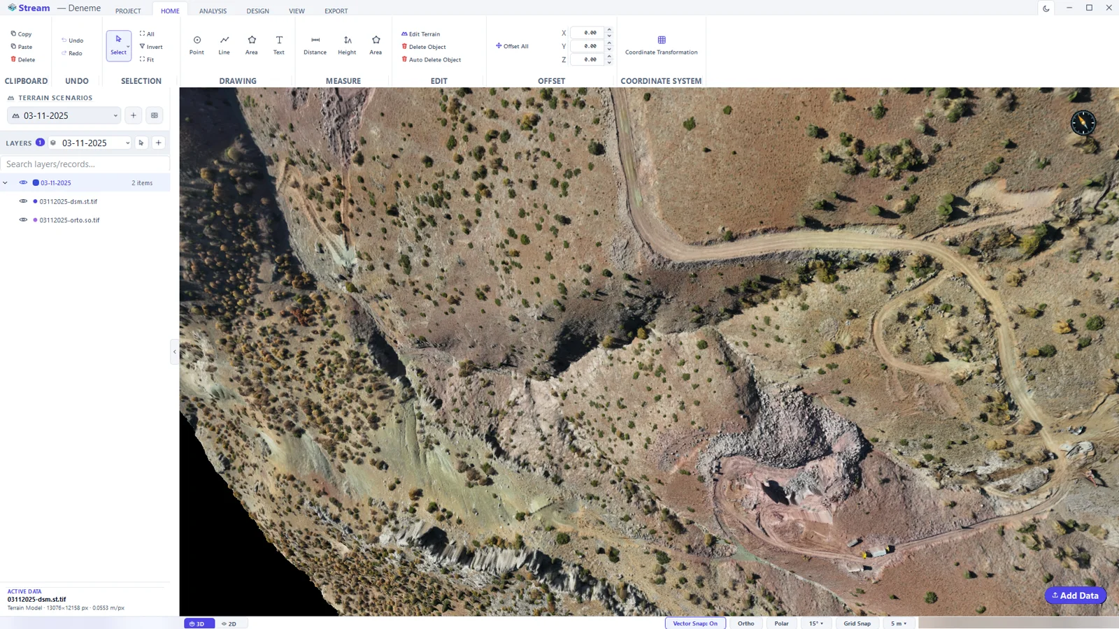
2D mode, 3D mode and camera direction
The VIEW tab controls the camera and what is shown around the map.

- 2D Mode locks the camera straight down, like a map sheet; orbit is switched off. 3D Mode frees it again. The same switch is in the status bar (3D / 2D).
- Face North turns the view north-up without changing the tilt. Top View looks straight down.
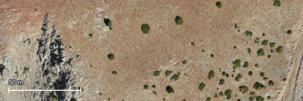
- Show Scale adds a scale bar to the view; Show Grid adds a coordinate grid. Show Left Panel and Fullscreen Mode hide the panels to leave more room for the map.
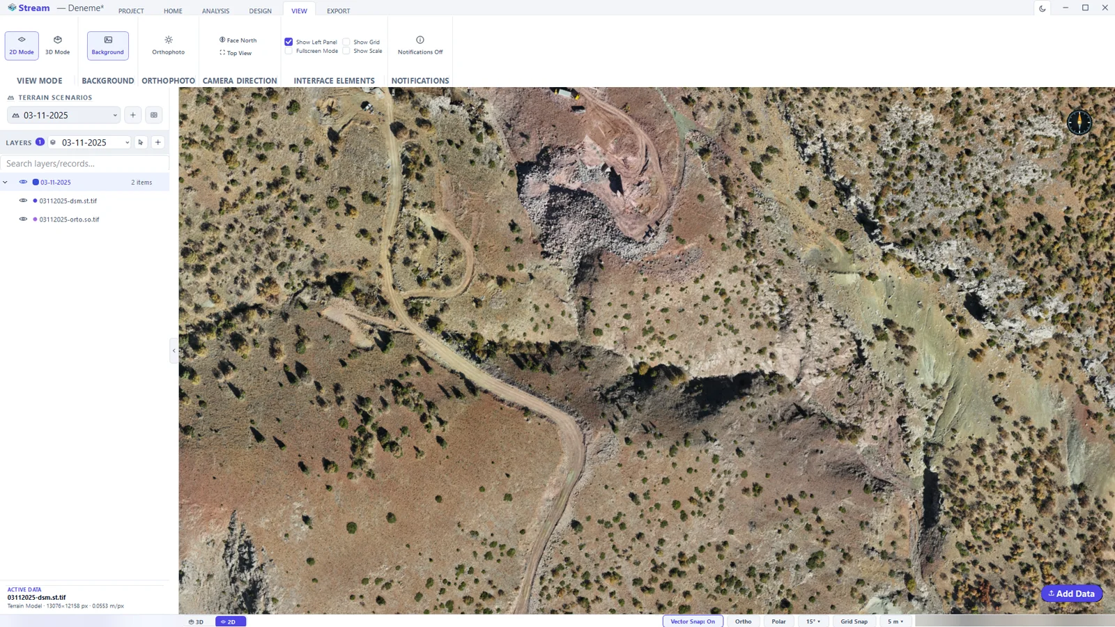
Background and Orthophoto on the same tab switch the backdrop colour and the draped imagery; Notifications Off / On controls the short information bubbles (off by default — error and confirmation dialogs always appear).
Light and dark theme
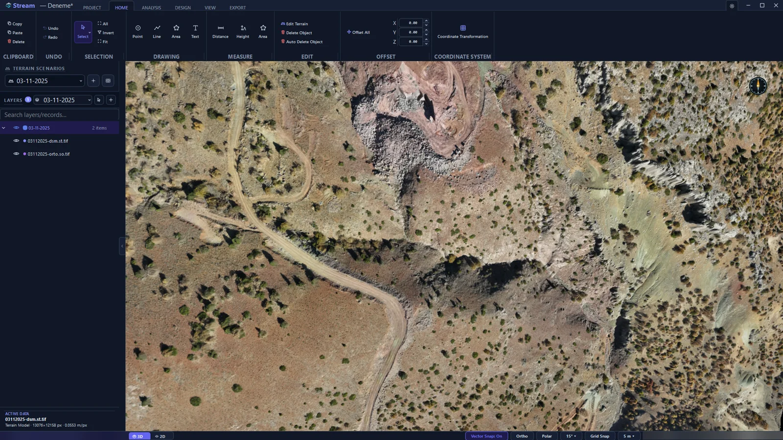
Click the moon button on the title bar (Dark / light theme) to switch. The whole interface redraws immediately; nothing needs a restart.
Terrain scenarios and layers
A terrain scenario is one state of the site: a survey date, a design stage, a before or an after. Keeping several scenarios in one project is what makes comparisons, cut/fill between two dates and change detection possible. The project in this manual holds two drone surveys of the same quarry.
Switching between scenarios
- Open the list under TERRAIN SCENARIOS in the left panel.
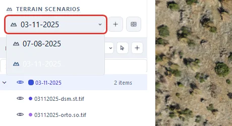
The scenario list: two surveys of the same site. - Pick a scenario. The view, the layer list and every tool now work on that survey.
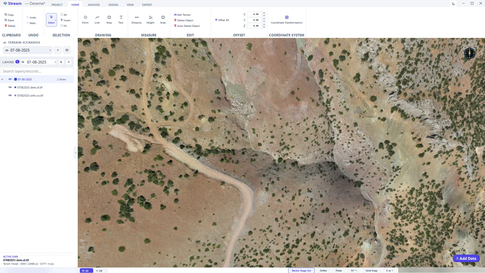
The earlier survey is now active: the quarry has not been opened yet. - Add Terrain Scenario (the + button next to the list) creates a new, empty scenario — load the next survey into it with Add Data.
The layer list
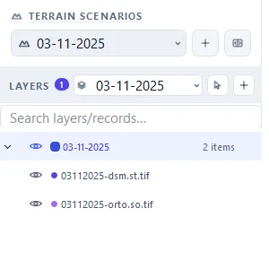
- The eye icon in front of a row shows or hides that layer or record.
- Click a row to select it; Ctrl-click selects several. Clicking a layer name selects everything in the layer.
- Right-click a record for Change Color, Attributes… and other actions.
- Pin a record to make it visible in every scenario; unpinned data is only shown in the scenario where it was created.
- Add Layer (the + button on the LAYERS row) creates a layer; the list next to it chooses the layer new drawings go into.
- Search layers/records… filters long lists.
Comparing two scenarios side by side
Compare Mode splits the view with a curtain: one scenario on the left, another on the right, same camera.
- Click Compare Mode, the button to the right of Add Terrain Scenario.
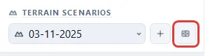
The Compare Mode button in the TERRAIN SCENARIOS row. - Choose the scenario for the left side (Ground) and for the right side (Reference), then press Compare.
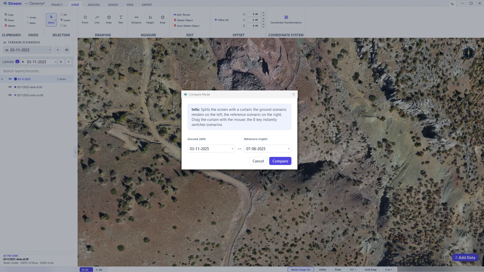
The Compare Mode dialog. - Drag the divider left or right. The camera stays where it is while the curtain moves. Press B to swap the two sides.
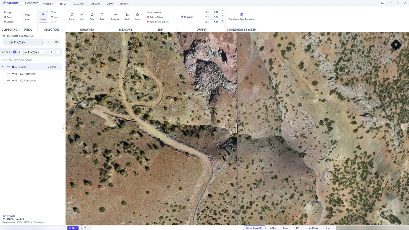
The curtain view: the later survey on the left, the earlier one on the right. - Click Compare Mode again to close the curtain.
Drawing
Points, lines, areas and text are drawn directly on the terrain: every vertex takes its elevation from the surface under the cursor.

The rules are the same for every tool: left click places a point or vertex, right click finishes the object, Esc cancels the one in progress, and a second right click leaves the tool.
Points
- Click HOME ▸ DRAWING ▸ Point. The POINT tab opens and the view shows Add Point active — click the terrain.
- Click the terrain. Each click places a point on the surface; X, Y and Z are read automatically.
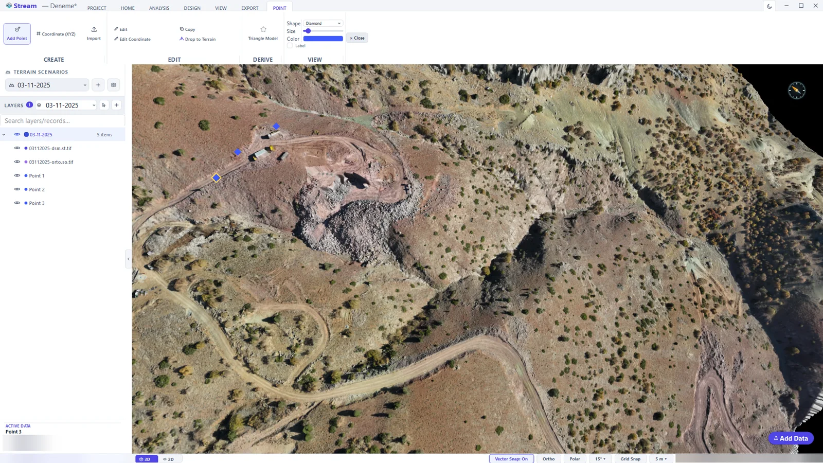
Three points placed on the terrain. Each one becomes a row in LAYERS. - To enter exact coordinates instead, use Coordinate (XYZ) on the POINT tab. Import reads a point list from a file.

With a point selected: Edit moves it with the mouse, Edit Coordinate changes it numerically, Copy duplicates it and Drop to Terrain snaps its elevation back onto the surface. Shape, Size, Color and Label change how it is drawn.
Lines
- Click HOME ▸ DRAWING ▸ Line.
- Click the terrain vertex by vertex.
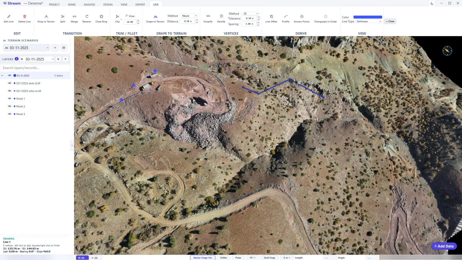
A line in progress: every click adds a vertex. - Right-click to finish. The line is selected, the LINE tab opens and ACTIVE DATA shows its 2D and 3D length, the bearing and the slope of the last segment.
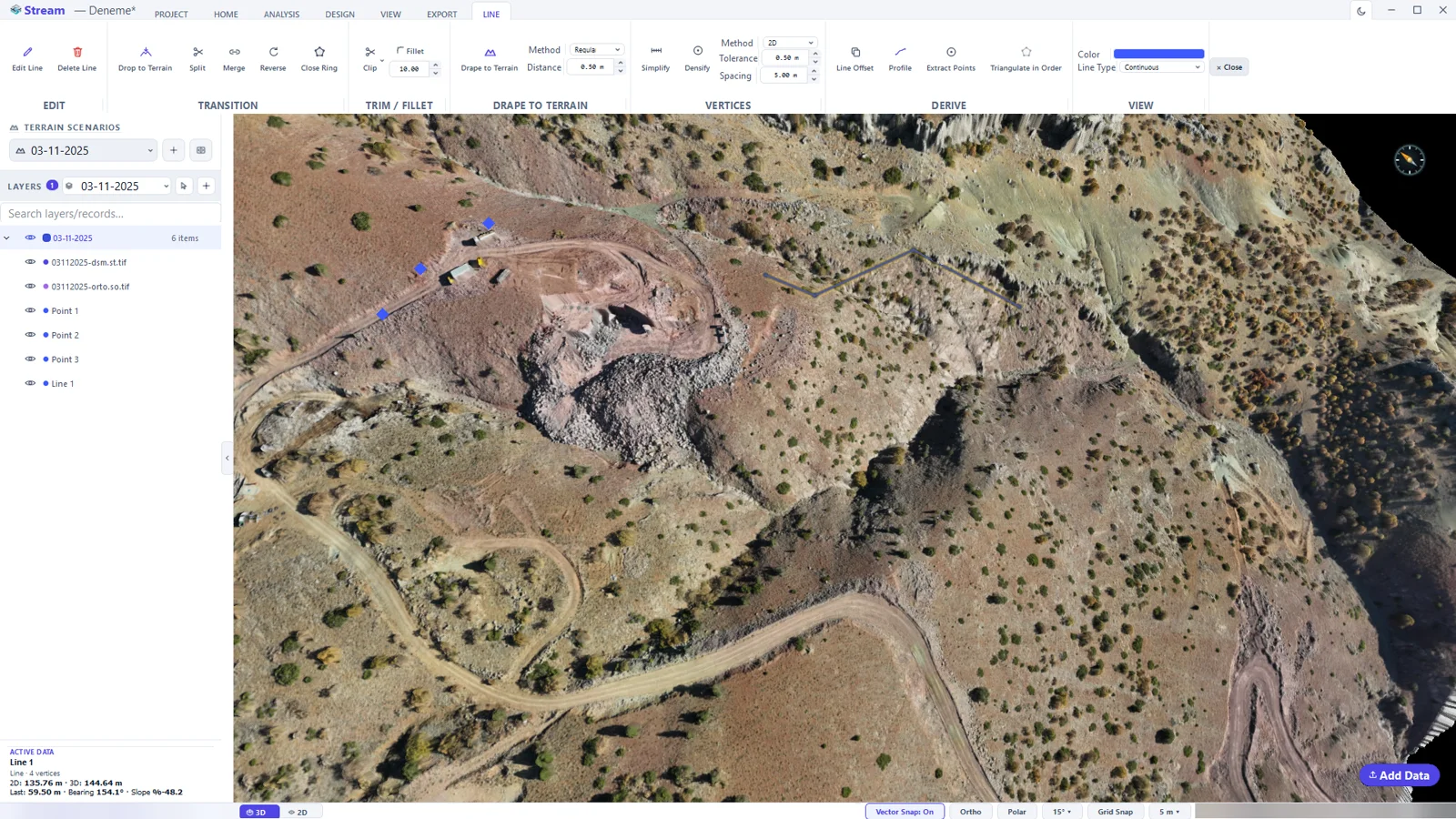
The finished line and its numbers in ACTIVE DATA.

- EDIT — Edit Line moves vertices, Delete Line removes the line.
- TRANSITION — Split cuts the line where you click, Merge joins two lines, Reverse flips the direction, Close Ring joins the last vertex to the first.
- TRIM / FILLET — Clip trims at a crossing line, Fillet rounds a corner with the given radius.
- DRAPE TO TERRAIN — beds the line onto the surface by sampling it at the given Distance.
- VERTICES — Simplify removes unnecessary vertices within the Tolerance; Densify inserts new ones at the given Spacing.
- DERIVE — Line Offset copies the line parallel at a distance, Profile draws the elevation profile along it, Extract Points turns the vertices into points.
Areas
- Click HOME ▸ DRAWING ▸ Area.
- Click the corners. While you draw, the card at the bottom-left shows the vertex count, the area and the perimeter so far.
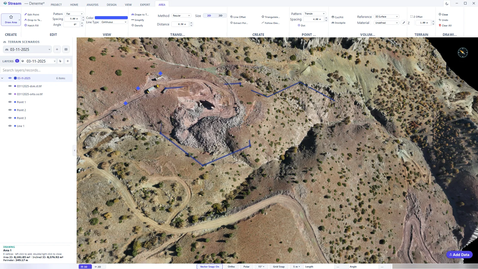
An area in progress. The DRAWING card updates with every corner. - Right-click to close the area. It is selected and the AREA tab opens.
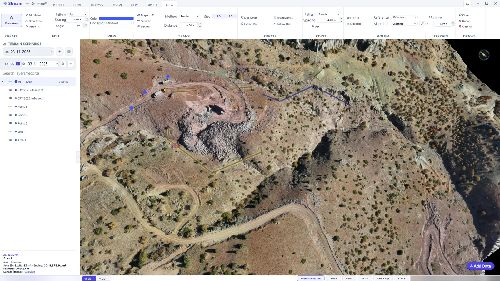
The closed area.

An area is the starting point of most calculations in STREAM — slope, contours, hydrology, cut/fill and stockpiles all work inside the selected area. The AREA tab also edits the shape itself:
- EDIT — Edit Point moves corners, Drop to Terrain beds the area onto the surface, Hatch Fill draws a hatch pattern instead of a solid fill.
- TRANSITION — Drape to Terrain, Simplify and Densify, as for lines.
- CREATE — Line Offset grows or shrinks a copy, Extract Points turns corners into points, Triangulate Inside builds a triangle model from the points inside, Follow Elevation turns the contour at the clicked elevation into an area.
- VOLUMES — Cut/Fill and Stockpile (see Volumes and change).
- ACTIVE DATA shows Area 2D, Inclined 3D (the area of the plane through the corners) and the perimeter. Click Calculate next to Surface (terrain) for the true draped surface area.
Text
- Click HOME ▸ DRAWING ▸ Text, then click the map where the text should sit.
- Type the text and press OK.
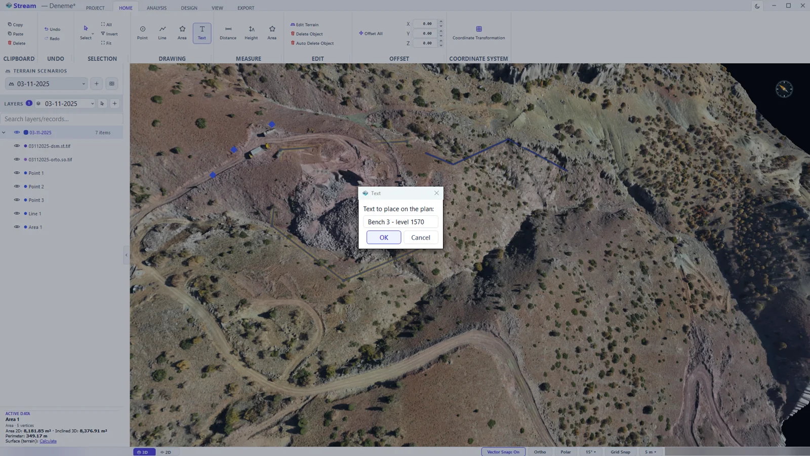
The Text dialog. - The text is placed on the plan and gets its own row in LAYERS.
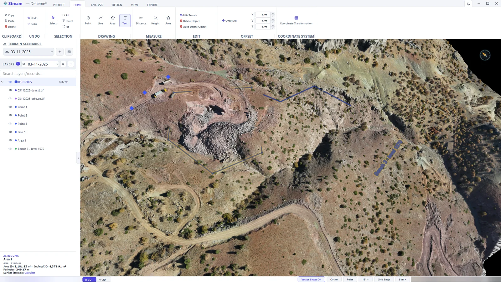
The text lies on the terrain and is listed in LAYERS.
While a text is selected, a TEXT group appears on the Selection tab: Edit Text changes the wording, Height is in metres (it grows as you zoom in and obeys the sheet scale when printed), Angle rotates it in plan.
Selecting and transforming
- Click HOME ▸ SELECTION ▸ Select (or leave the active tool with a right click), then click an object. Ctrl-click adds to the selection.
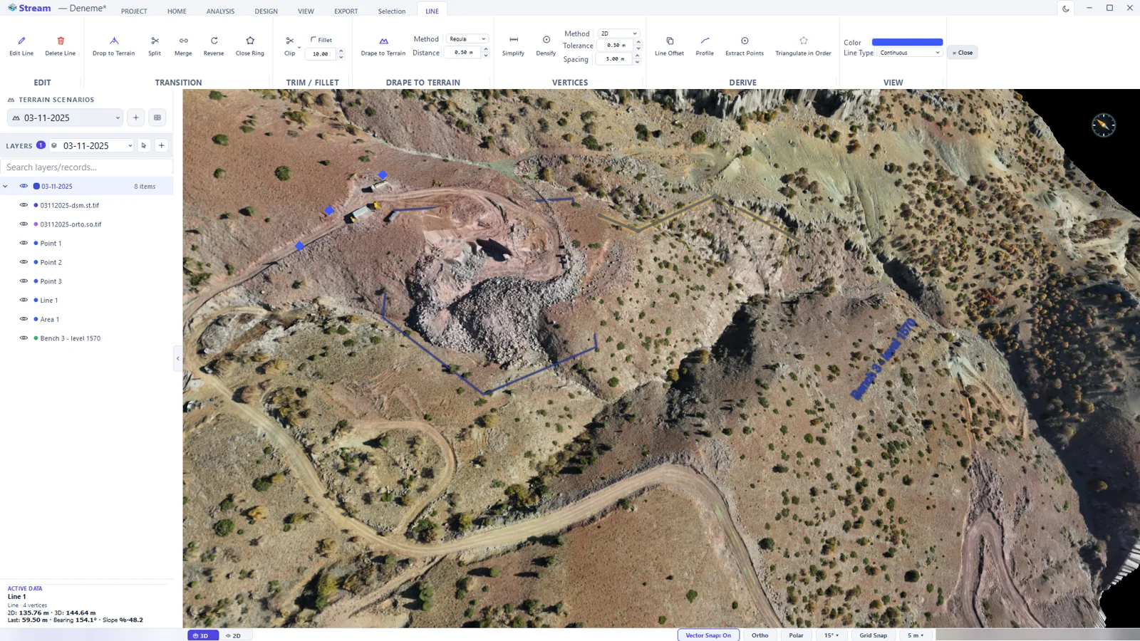
One click selects the line; its context tab opens. - All selects every point, line and area; Invert swaps the selection. Fit frames all loaded data on screen.
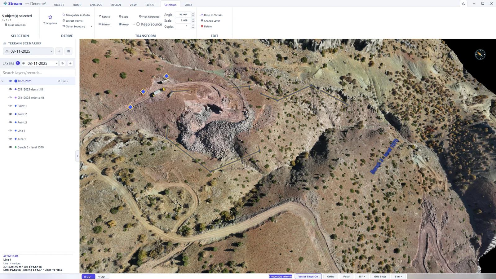
Everything selected: the Selection tab counts points, lines and areas. - The Selection tab works on all selected objects at once: Rotate, Mirror, Scale and Array under TRANSFORM (tick Keep source to work on a copy), Outer Boundary to wrap them in a new area, Change Layer, Drop to Terrain and Delete.
Measuring
The three tools in HOME ▸ MEASURE measure live on the terrain. Nothing has to be drawn first.

Distance
- Click Distance and click along the path you want to measure.
- The running total follows the cursor in the view; the ACTIVE MEASUREMENT card shows the 2D Length (horizontal) and the 3D Length (along the slope).
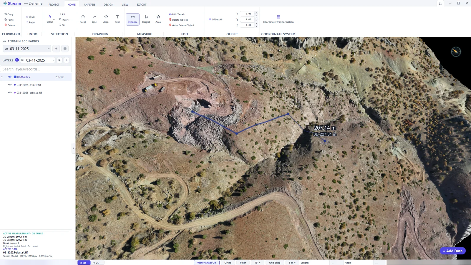
A distance measurement in progress. 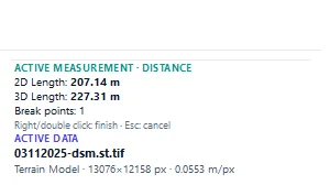
The ACTIVE MEASUREMENT card. - Right-click to finish — the measurement is added to LAYERS — or press Esc to discard it.
Height
- Click Height, then click the first point.
- Move to the second point: the elevation difference and the slope between the two are shown live. Click to fix it.
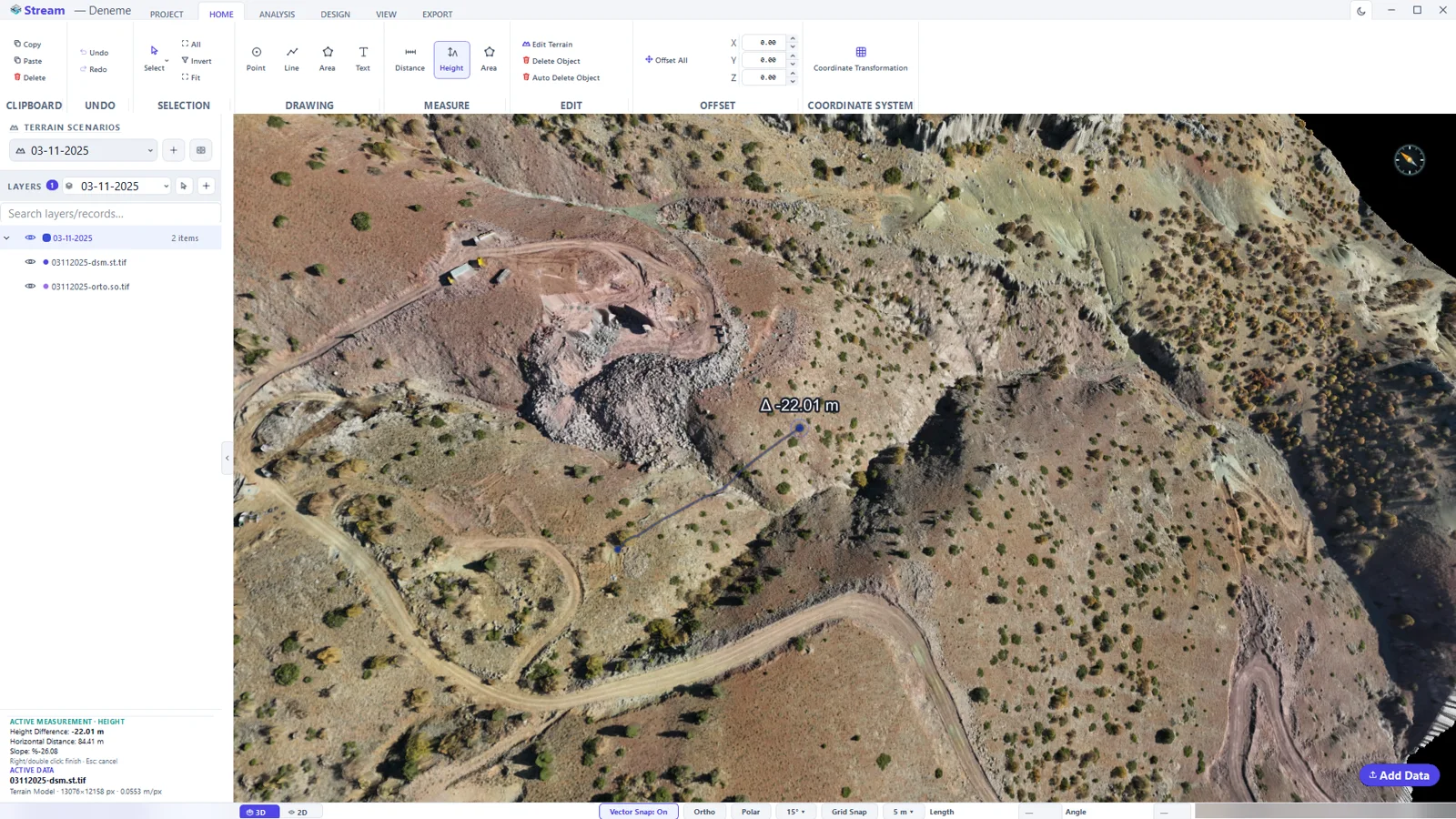
Height: the elevation difference between two points.
Area
- Click Area in the MEASURE group and click the corners.
- The label in the view and the card show the 2D Area, the 3D Area and both perimeters.
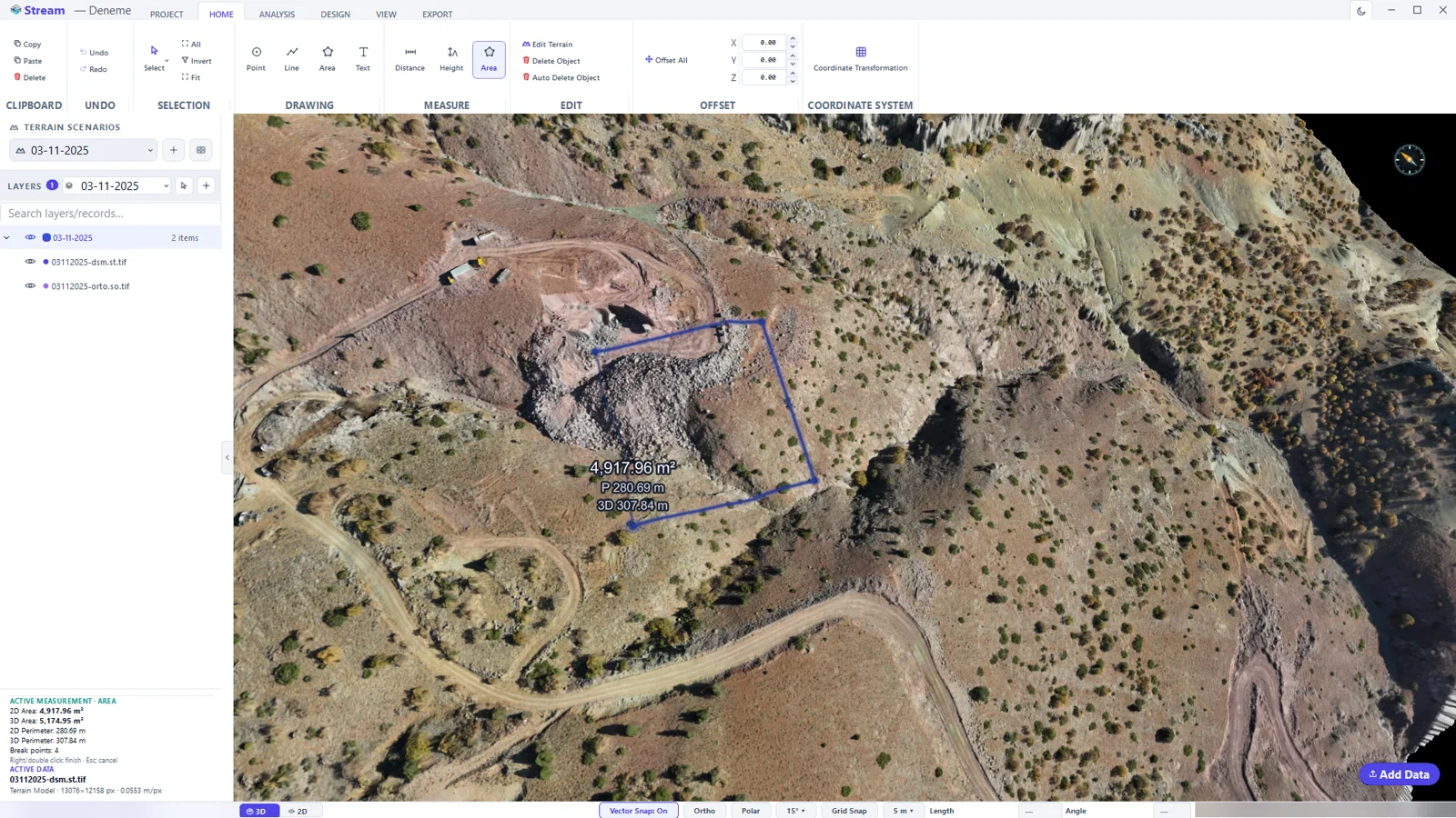
An area measurement: plan area, surface area and perimeter. - Right-click to finish or Esc to discard.
Analysing the terrain
The ANALYSIS tab turns the surface into answers: how steep, which way it faces, what can be seen from where, where water goes, how much sun it gets.

Most analyses share the same three habits:
- They work inside an area. Draw an area first (HOME ▸ DRAWING ▸ Area) and keep it selected; the context tab then shows Scope: Area 1. Change Area and Select Area on every analysis tab switch to another one.
- The result is live. A coloured overlay is painted on the terrain as soon as the tool opens and follows every setting you change.
- You decide what to keep. Add to Layer keeps the overlay as a record, Add as Raster writes a georeferenced image, Add as Vector turns it into drawing geometry. × Close leaves the tool without keeping anything.
Slope
- Select an area and click ANALYSIS ▸ TOPOGRAPHY ▸ Slope.
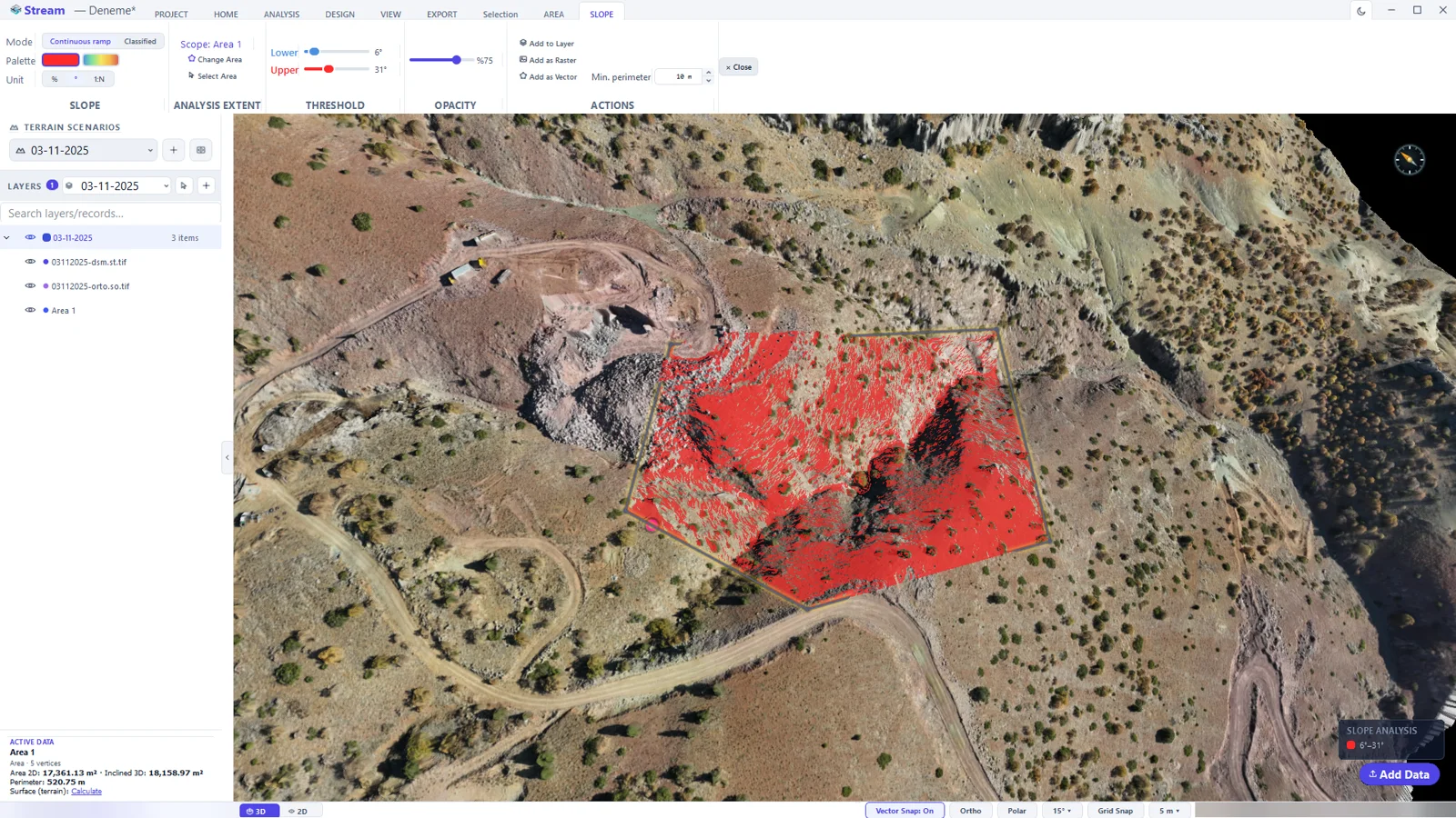
Slope: everything between the lower and upper threshold is painted. - On the SLOPE tab set the Lower and Upper threshold to isolate a slope range — for example everything steeper than the angle a machine can work on.

The SLOPE tab: mode, palette, unit, analysis extent, threshold, opacity and actions. - Unit switches between percent (%), degrees (°) and ratio (1:N). Palette chooses a single colour or a rainbow ramp. Opacity lets the orthophoto show through.
- Switch Mode to Classified to split the area into slope classes instead of a continuous ramp; choose the Method and the Class count.
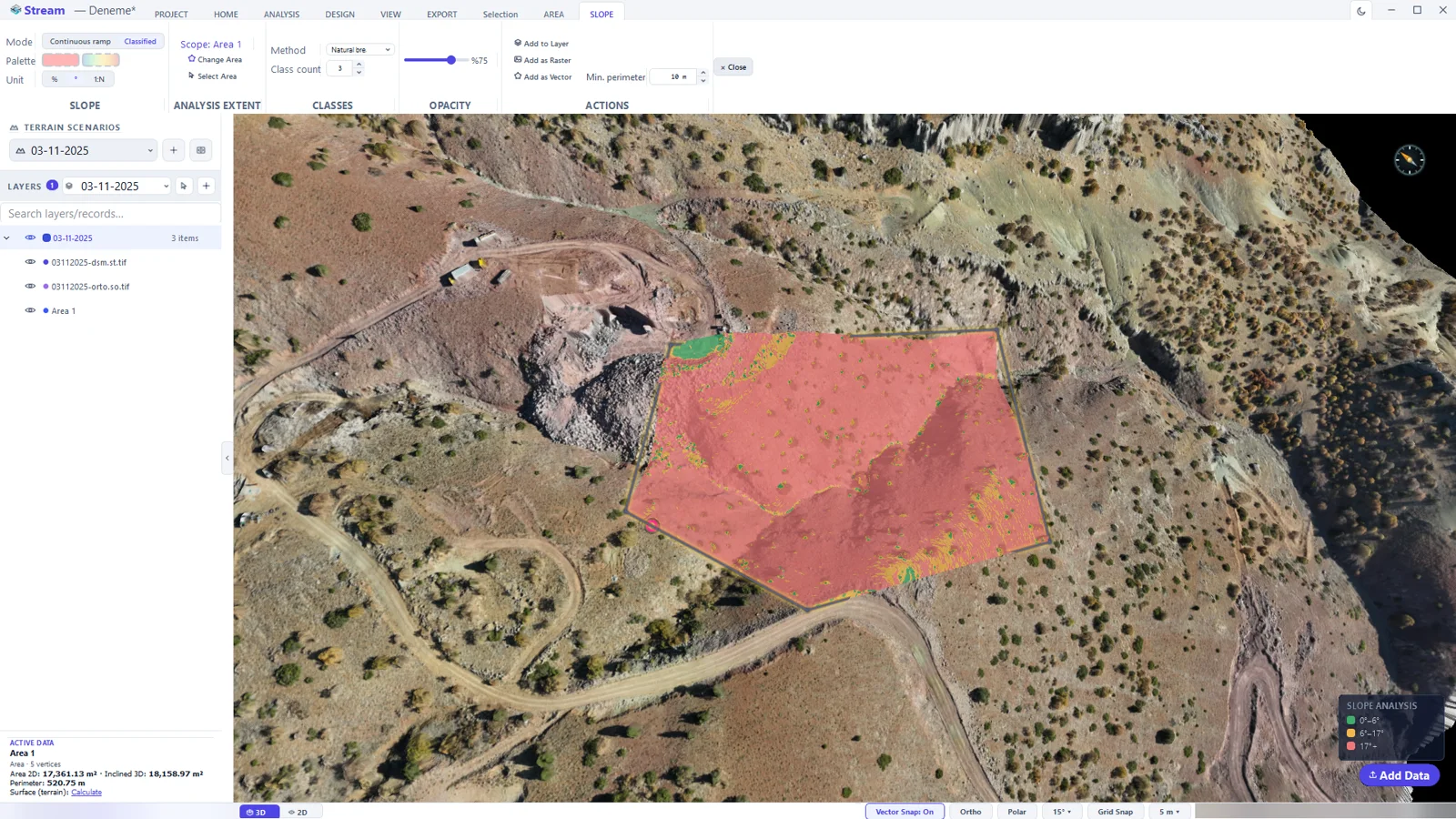
Classified mode: the area split into slope classes.
Aspect
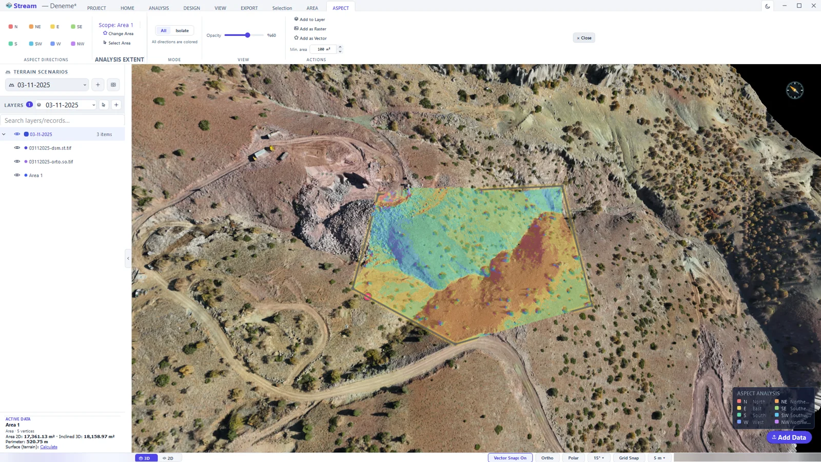
Aspect colours the direction each slope faces. Click one of the eight direction buttons (N, NE, E …) and choose Isolate to show a single direction — the north-facing ground that keeps snow, or the faces that get the afternoon sun.
Shading
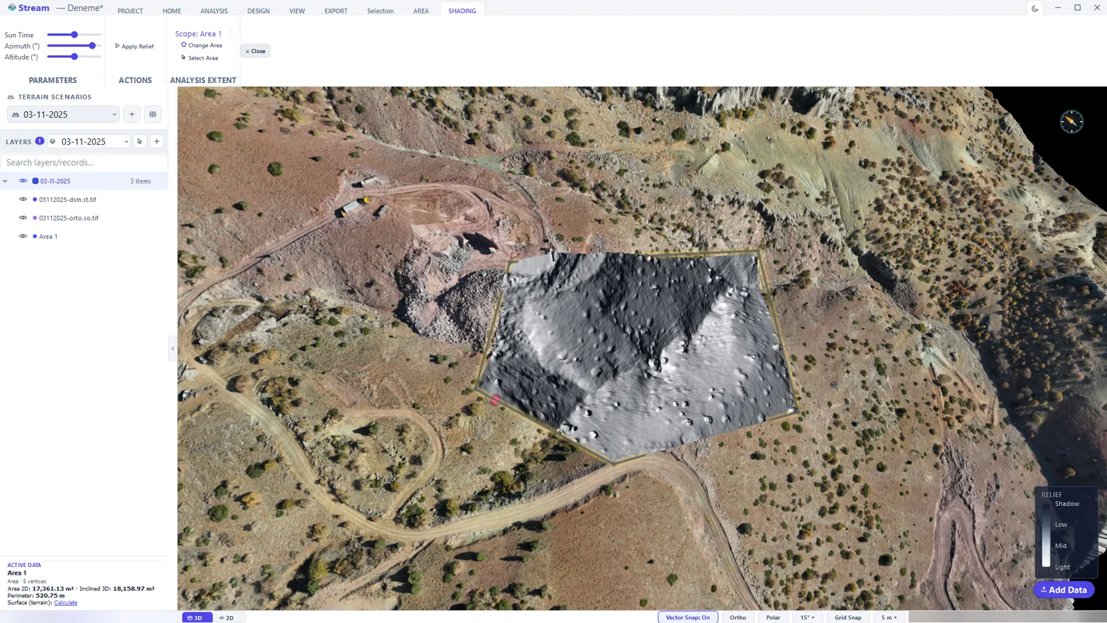
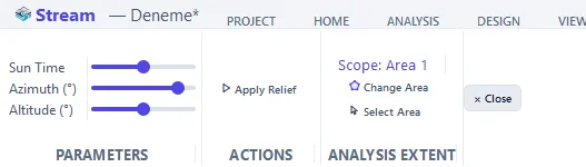
Shading lights the relief from a direction you choose. Drag Sun Time, or set Azimuth and Altitude directly; Apply Relief keeps the result.
Contours
- Select an area and click ANALYSIS ▸ TOPOGRAPHY ▸ Contours. Contour lines are drawn inside the area straight away.
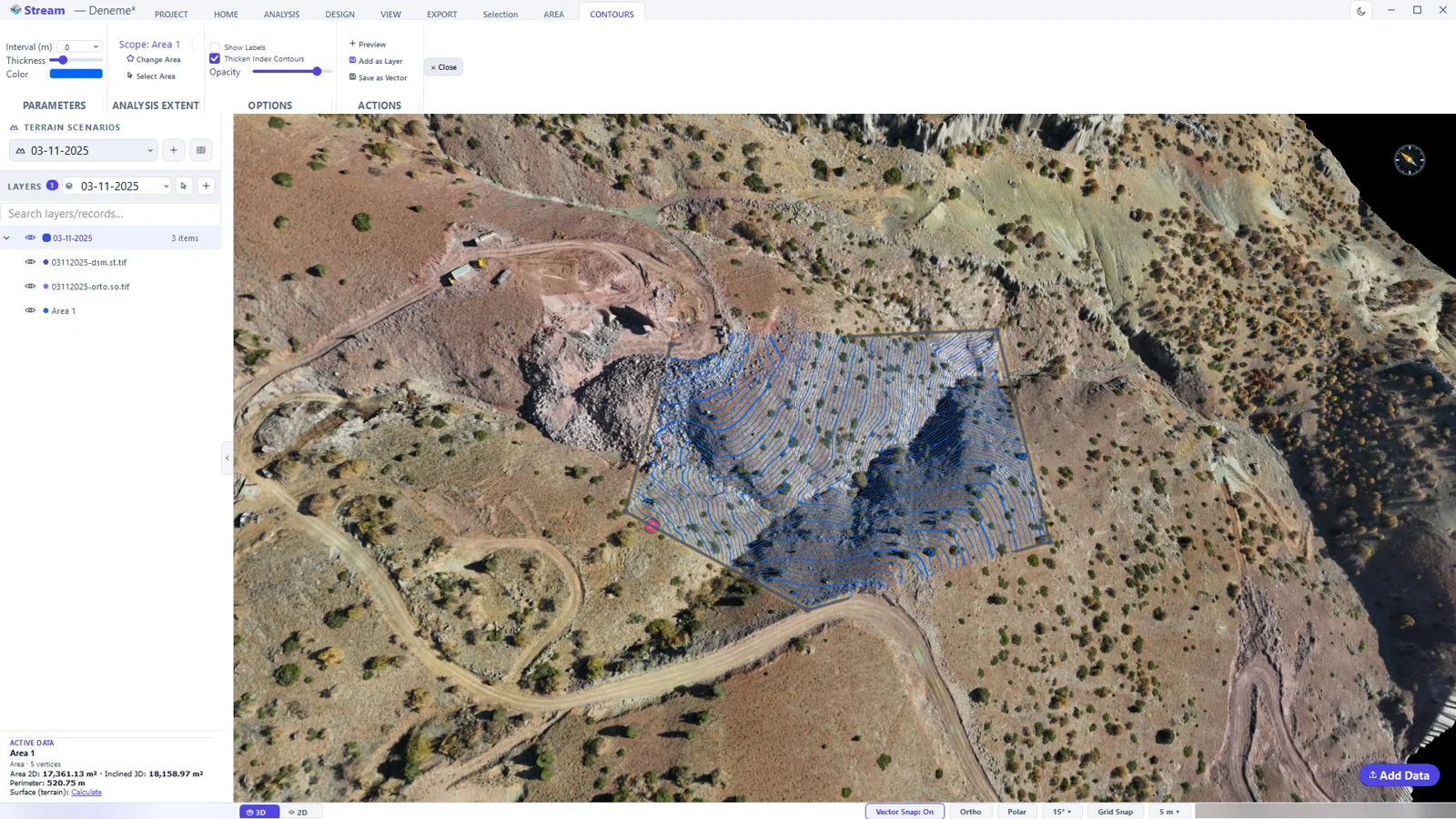
Contours generated inside the selected area. - Set the Interval (m), the line Thickness and Color. Thicken Index Contours draws the index contours heavier; Show Labels writes the elevations.
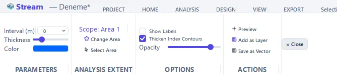
The CONTOURS tab. - Add as Layer keeps the contours in the project; Save as Vector writes them to DXF for CAD.
Viewshed and line of sight
Viewshed answers “what can be seen from here?”
- Select an area, click ANALYSIS ▸ TOPOGRAPHY ▸ Viewshed, then click the terrain where the observer stands.
- Visible ground is painted green, hidden ground red. Height is the observer's eye height; Radius limits the sight distance (0 = unlimited).
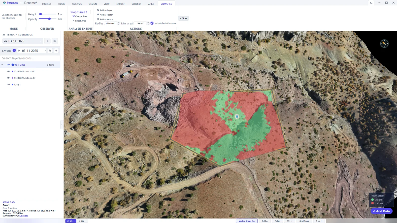
Viewshed from the clicked observer point: green is visible, red is hidden.
Line of Sight tests a single sight line between two points.
- Click ANALYSIS ▸ TOPOGRAPHY ▸ Line of Sight, press New Line, then click the observer and the target.
- The line is drawn green where the target is visible and red behind the first obstruction. The panel at the bottom shows the terrain profile under the line with the sight line on top.
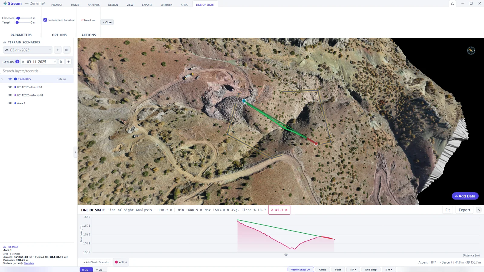
Line of Sight: the sight line on the map and its profile below.
Profile
- Click ANALYSIS ▸ PROFILE ▸ Profile and draw the section line on the terrain; right-click to finish.
- The SECTION PROFILE panel opens under the view: length, lowest and highest elevation, average slope and elevation difference in the header; total ascent and descent at the bottom.
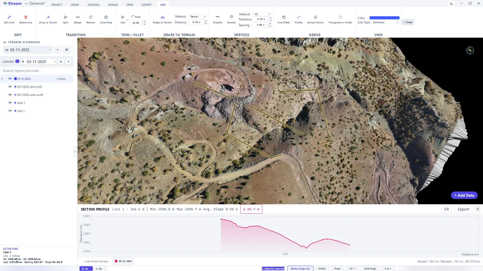
A section profile along the drawn line. - + Add Terrain Scenario overlays the same section from another scenario — the quickest way to see what changed between two surveys along a line.
- Export writes the profile out; Fit resets the chart zoom.
Hydrology
- Select an area and click ANALYSIS ▸ WATER & DRAINAGE ▸ Hydrology. The HYDROLOGY tab opens in Watershed mode: each drainage basin gets its own colour, and the card at the bottom-left counts the basins and reports the stream length, the drainage density and the longest flow path.
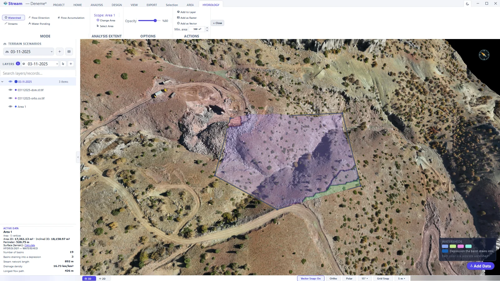
Watershed mode: drainage basins inside the area and their summary. 
The HYDROLOGY tab. - Switch the mode to read the same surface differently:
- Flow Direction — the steepest descent direction of every cell.
- Flow Accumulation — how much upstream area drains through each cell.
- Streams — the stream network; Stream Threshold sets how much upstream area makes a stream (automatic by default).
- Water Ponding — the closed depressions where water collects, with their depth and storage volume. Here you can also enter a Rainfall or a Return period to see which depressions fill.
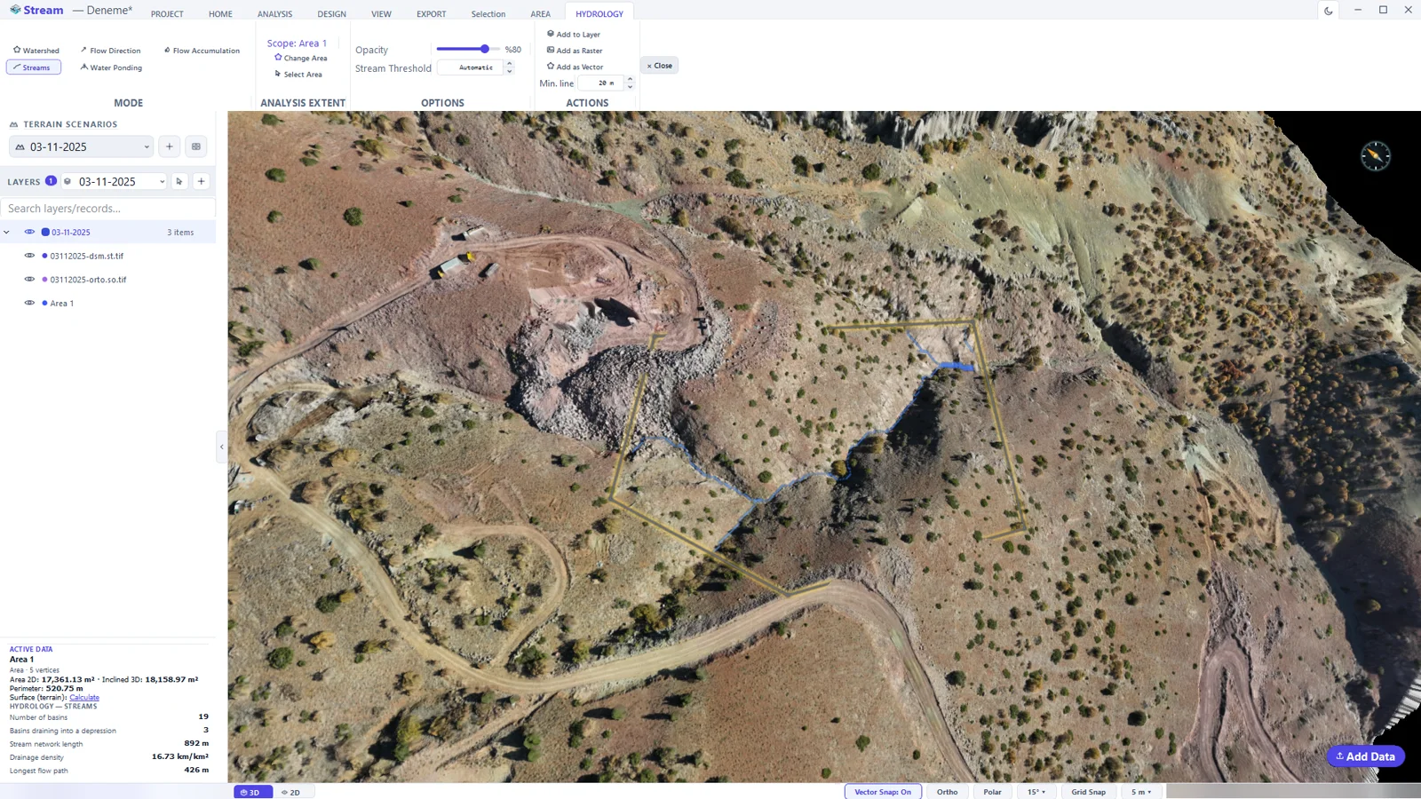
Streams mode: the derived stream line inside the area. - Click the terrain in Watershed mode to get the catchment draining to that point.
Sun & Shadow
Sun & Shadow computes how many hours of sun each part of the site receives, including the shadow thrown by the surrounding hills.
- Select one or more areas and click ANALYSIS ▸ SURFACE ANALYSIS ▸ Sun & Shadow. The panel opens under the view.
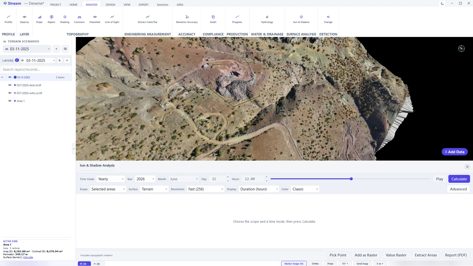
The Sun & Shadow panel before the calculation. - Choose the Time mode: Instant (one day and hour), Daily, Monthly or Yearly. Set Scope to Selected areas or the whole terrain and pick a Resolution.
- Press Calculate.
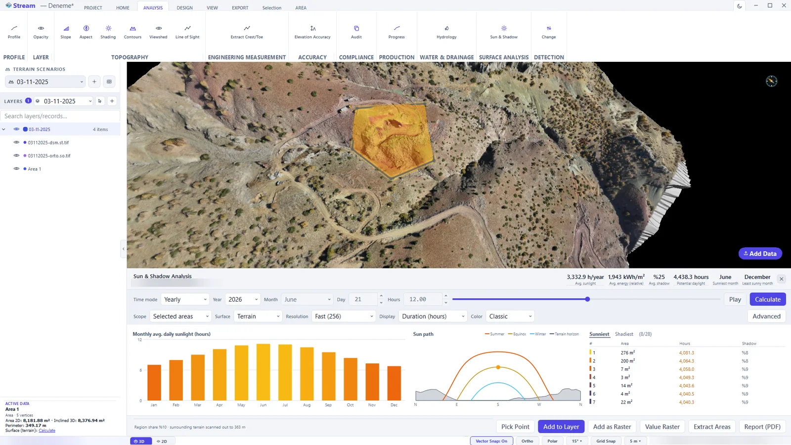
The yearly result: the map, sunlight per month, the sun path with the terrain horizon, and the sunniest regions. - Read the result: the header gives the average sunlight, energy and shadow share; the bar chart shows the average daily sunlight per month; Sun path shows the summer, equinox and winter arcs above the terrain horizon; the table lists the sunniest and shadiest regions — click a row and the map goes there.
- Display switches the map between duration, energy and shadow ratio without recomputing. Pick Point shows the first and last sun time of a point you click.
- Keep the result with Add to Layer, Add as Raster, Value Raster (a GeoTIFF with the numbers), Extract Areas or Report (PDF).
Volumes and change
This is the reason most sites buy a drone: how much material moved between two surveys, how much is in that pile, and where exactly the ground changed. All three start from an area and a reference.
Cut and fill between two surveys
- Make the later survey the active scenario and draw an area around the place you want to quantify (HOME ▸ DRAWING ▸ Area). Keep it selected: the AREA tab stays open.

The AREA tab. The VOLUMES group (1) holds Cut/Fill, Stockpile and the reference settings. - In the VOLUMES group open Reference — the surface the area is compared against:
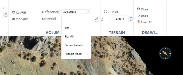
The Reference list. - 3D Surface — a surface stretched through the corners of the area.
- Flat — a fixed elevation you type.
- Flat Min — a flat base at the lowest elevation in the area.
- Terrain Scenario — another survey of the same site.
- Triangle Model — your own design surface (TIN).
- Choose Terrain Scenario, pick the earlier survey in Scenario, and press Cut/Fill.

1 — Reference, 2 — Scenario, 3 — Cut/Fill. - The result is painted inside the area in two colours, and a new record appears in LAYERS, named after the area and the reference.
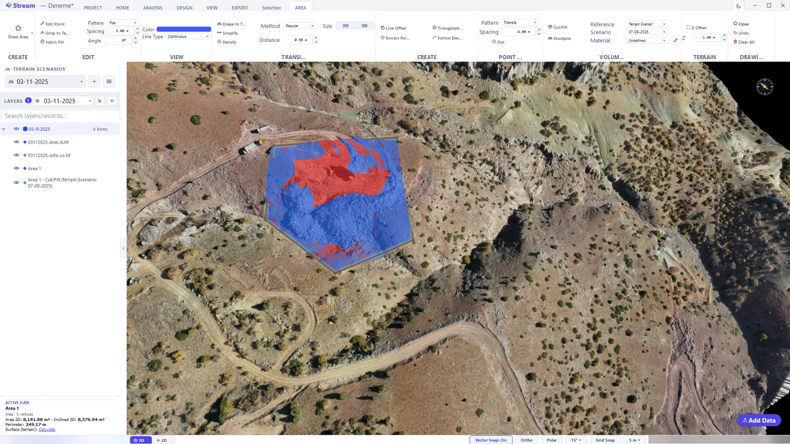
Cut and fill between the two surveys, painted inside the area. Cut (blue) is where the active surface lies above the reference; fill (red) is where it lies below it. In this example the reference is the earlier survey, so the heap dumped since then counts as cut and the pit excavated since then counts as fill.
- Click the map with the Select tool. ACTIVE DATA now shows the numbers: Cut volume, Fill volume, Net cut/fill and the Area. The status bar reads the cut or fill depth under the cursor.
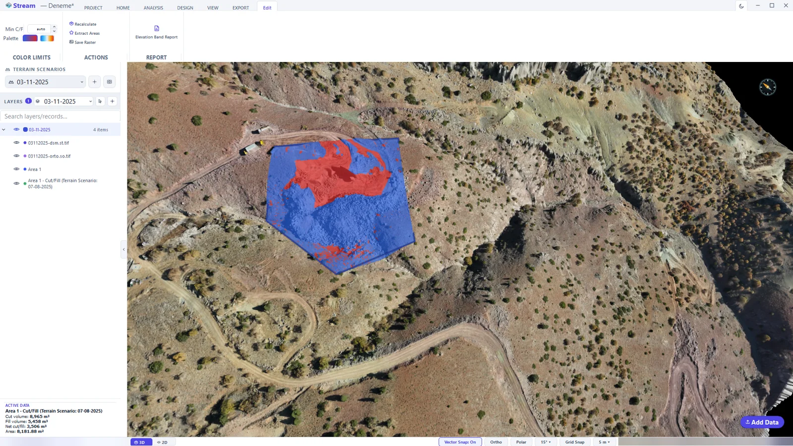
The cut/fill map selected: its Edit tab is open and the volumes are in ACTIVE DATA. 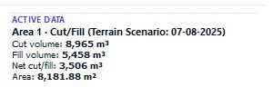
The volume card. - The Edit tab of the map holds the follow-up actions:
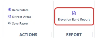
Actions and report on the Edit tab of a cut/fill map. - COLOR LIMITS ▸ Recalculate repaints the map with your own lower and upper limit and band count.
- Extract Areas turns the cut and fill boundaries into editable areas.
- Save Raster writes the map to a GeoTIFF.
- Elevation Band Report splits the volume into elevation bands.
Elevation Band Report
“Floor level 1560, every 10 metres — how much cut and fill is in each band?” The Elevation Band Report answers that from the cut/fill map you already have.
- Select the cut/fill map and press Elevation Band Report on its Edit tab.
- Choose the Band height — 5 m, 10 m or Custom. No table is produced until you choose; the bench height of your site is the natural value.
- Leave Floor level and Top level on auto to cover the whole range where material exists, or type your own levels. Tick Add cumulative columns to sum from the floor up.
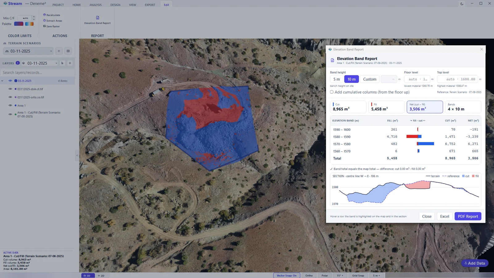
The Elevation Band Report for the cut/fill map. - Excel writes the table on screen; PDF Report adds the elevation–volume chart, the site view and the method notes.
Stockpiles
A stockpile uses the same volume engine, but the result becomes a pile record with a material attached: density gives tonnage, unit price gives value.
- Trace the toe of the pile with HOME ▸ DRAWING ▸ Area.
- On the AREA tab choose the Reference — the base the pile sits on. Flat Min uses the lowest corner; 3D Surface stretches a base through the corners, which suits a pile on sloping ground.
- Choose the Material (or leave it Undefined — the volume is still correct, only tonnage and value are left out) and press Stockpile.

1 — Reference, 2 — Material, 3 — Stockpile. - The pile is painted and added to LAYERS.
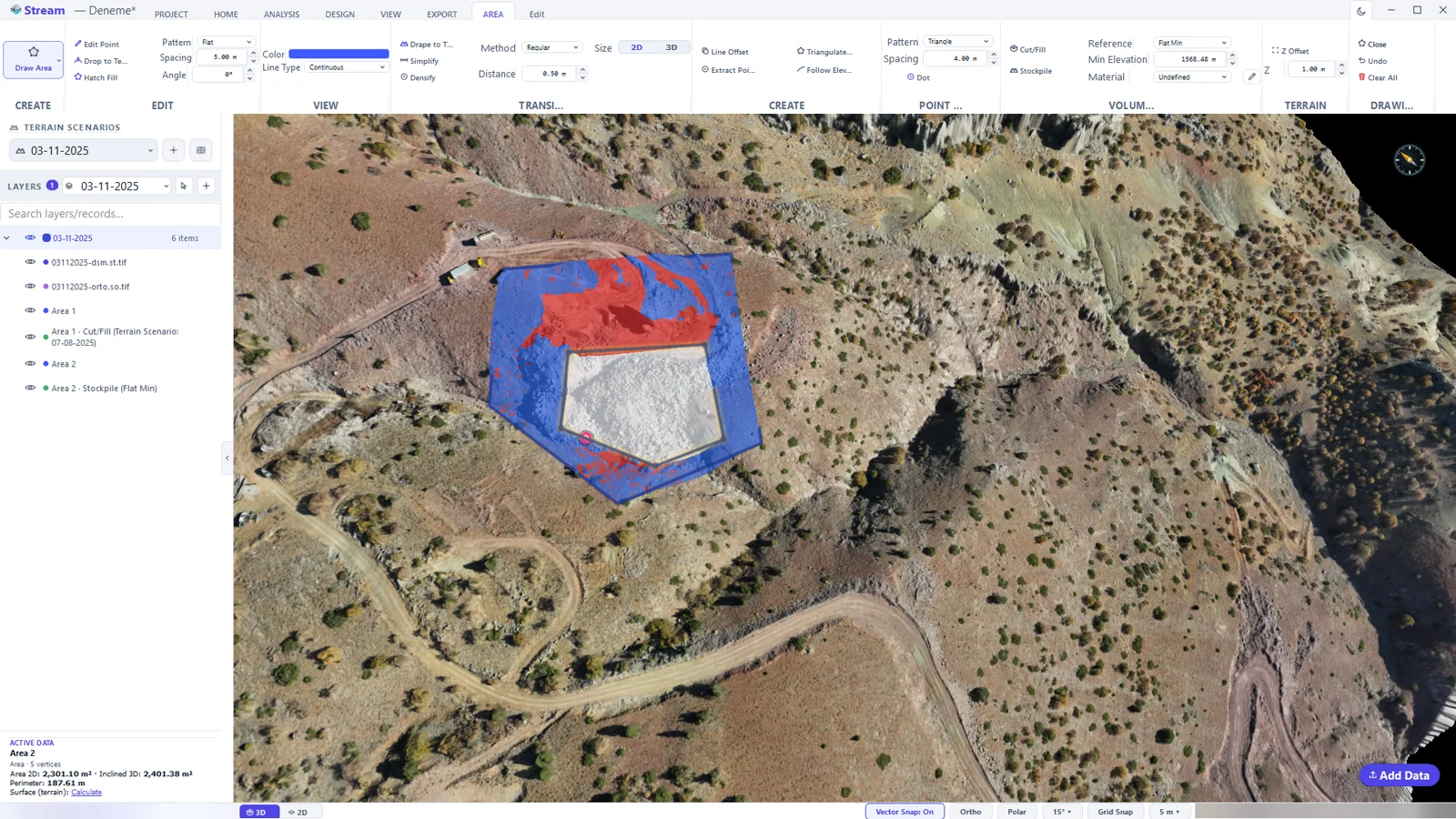
A stockpile measured against a flat base at its lowest point. - The pencil button next to Material opens the material library: name, colour, density (t/m³) and unit price for each material.
- EXPORT ▸ REPORTING ▸ Stockpile Report collects every pile on the site into one PDF.
Change Detection
Change Detection compares two surveys and separates real change from survey noise.
- Make the later survey the active scenario and draw an area around the place you want to check.
- Select the area: with the Select tool click its outline. The Selection tab appears. Change Detection needs exactly one selected area.
- Click ANALYSIS ▸ DETECTION ▸ Change. A short list of the other scenarios opens — pick the earlier survey; it becomes the before state.

The Change button on the ANALYSIS tab. - Only the ground that really changed is painted: orange to red where material was removed, blue where it was added. Everything below the detection threshold stays untouched. A Change Detection record is added to LAYERS.
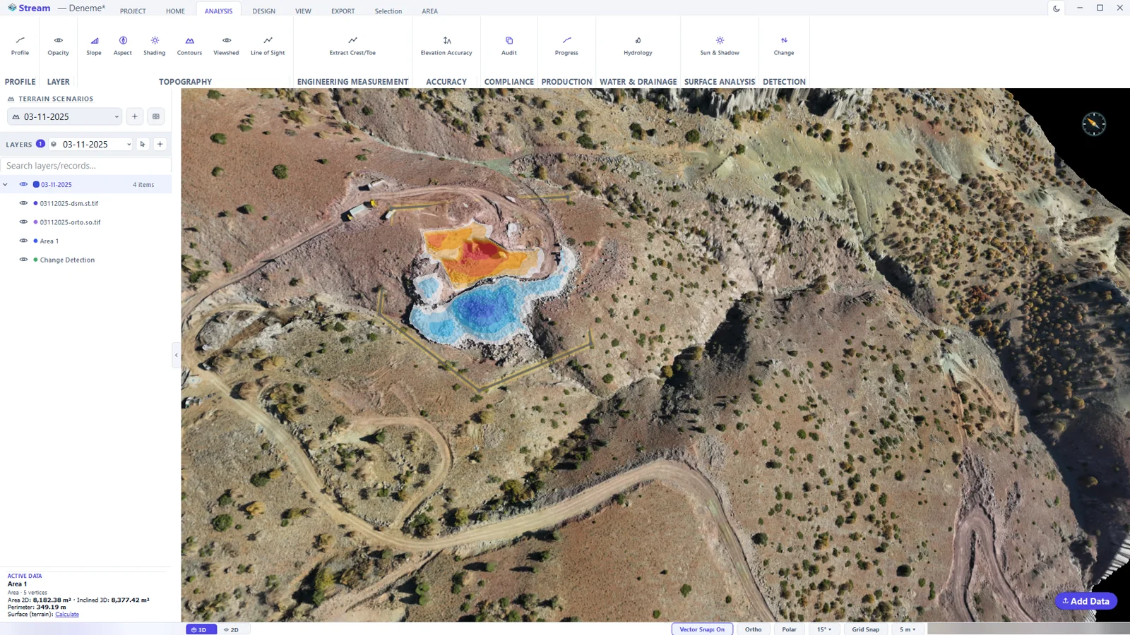
Change Detection between the two surveys: the excavation in orange and red, the new spoil heap in blue. - Click the map with the Select tool. ACTIVE DATA reports Deposition, Erosion, the Net volume with its ± uncertainty, the Changed area, the Detection threshold (LoD) and the number of Change regions.
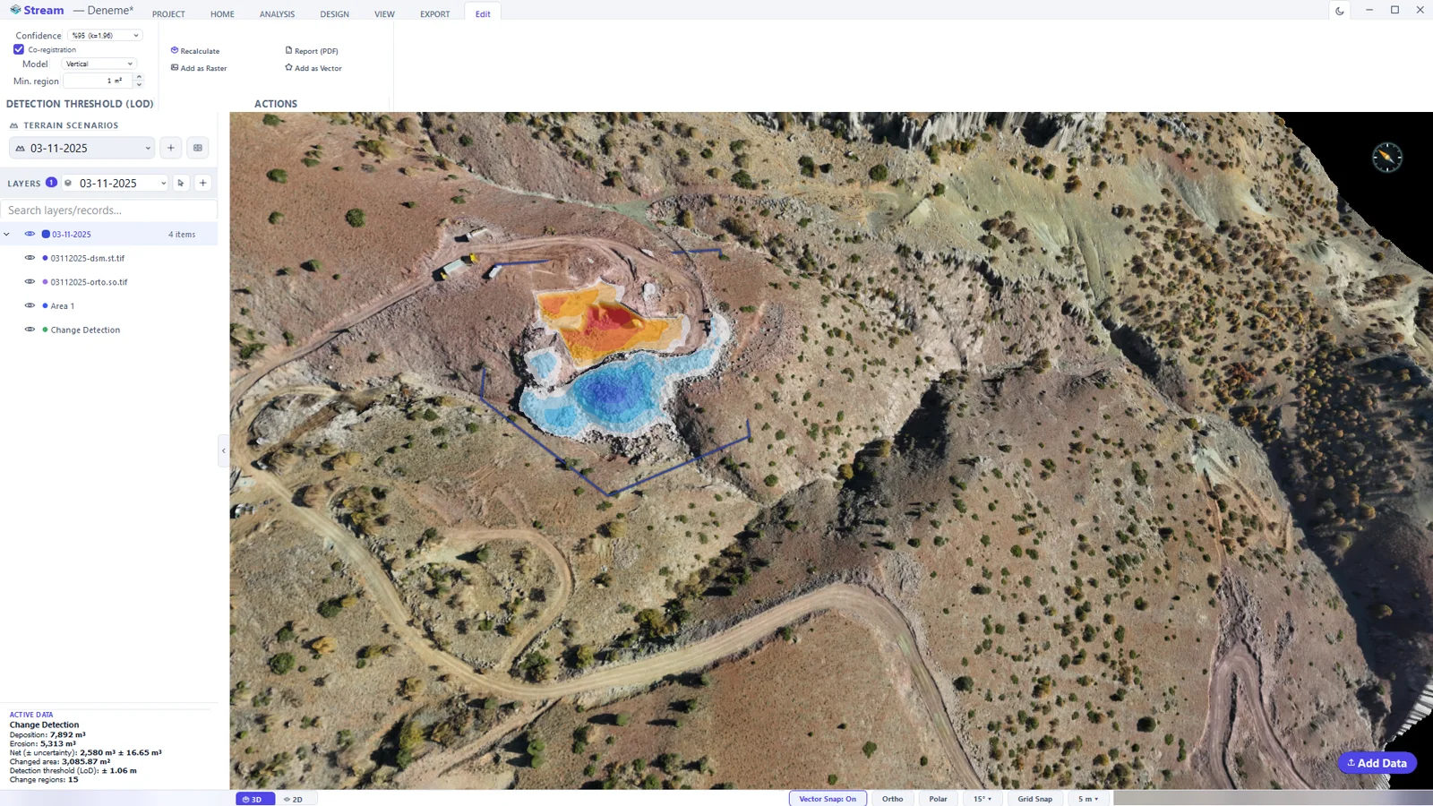
The change map selected: its Edit tab and the volume card. 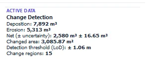
The Change Detection card. - The Edit tab tunes the analysis and exports it:
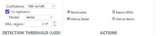
The Edit tab of a change map. - Confidence sets the detection threshold: differences smaller than it are treated as survey noise, not change.
- Co-registration removes a systematic shift between the two surveys before they are compared; Model chooses whether only a vertical shift or also a tilt is removed.
- Min. region drops change patches that are too small to be real.
- Recalculate applies the settings. Add as Raster, Add as Vector and Report (PDF) keep the result.
Engineering tools
Crest and toe extraction
Extract Crest/Toe finds every slope face by itself and adds the crest (top of slope) and the toe (bottom of slope) as 3D lines — hours of CAD work in one command.
- Click ANALYSIS ▸ ENGINEERING MEASUREMENT ▸ Extract Crest/Toe.
- Choose where it should run: draw a boundary, use the selected area, or scan the whole map. A smaller area gives a finer result.
- The lines are written to two layers, Crest and Toe. Ramp and haul-road edges are kept apart in Ramp Crest and Ramp Toe, so a road edge is never mistaken for a bench face.
- Each line is an ordinary line: select it, edit it, undo it, export it to DXF. Crest 3 and Toe 3 are the two edges of the same face.
Elevation accuracy
Elevation Accuracy documents how closely a surface matches points of known elevation — ground control points, levelling or GNSS measurements.
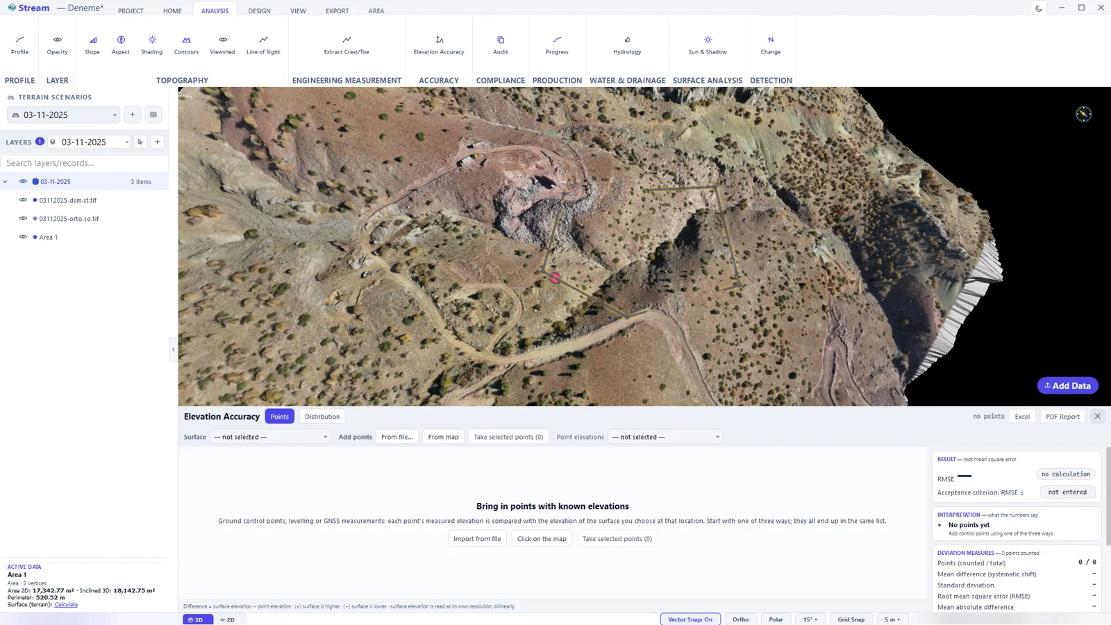
- Click ANALYSIS ▸ ACCURACY ▸ Elevation Accuracy. The panel opens under the view.
- Choose the Surface the points are compared against. Nothing is computed until you choose.
- Bring in the points: From file… (CSV or TXT with name, X, Y and the measured elevation), From map (click and type the measured elevation) or Take selected points.
- For every point the panel shows surface elevation − point elevation and summarises the result as RMSE. Enter an acceptance criterion to get a pass or fail verdict.
- Excel and PDF Report write the table and the report.
Coordinate transformation
Coordinate Transformation moves the whole project — points, lines, areas, text, rasters and terrain corrections together — into another coordinate system.
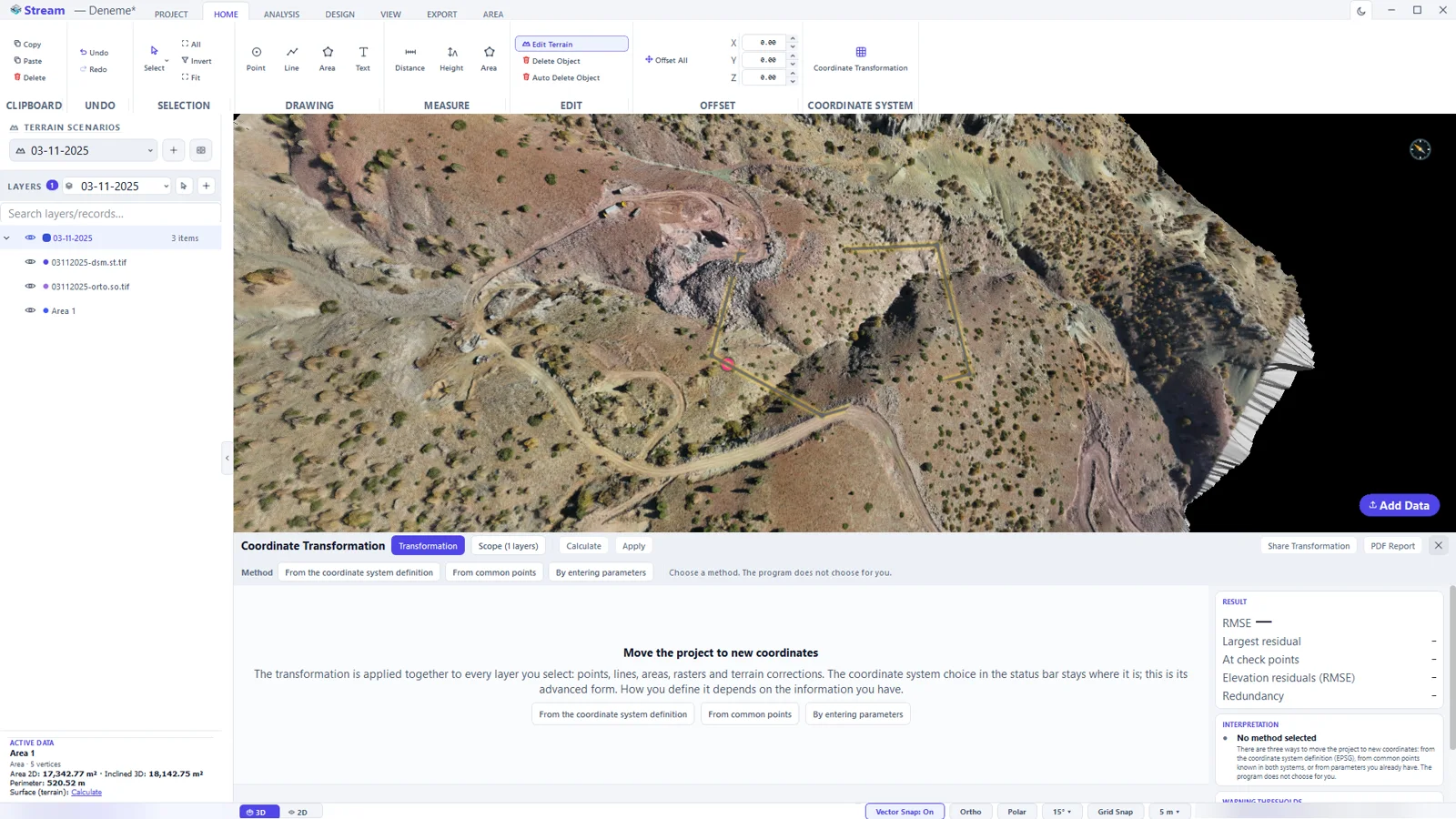
- Click HOME ▸ COORDINATE SYSTEM ▸ Coordinate Transformation.
- Choose the Method:
- From the coordinate system definition — both systems are known (EPSG); you pick the target.
- From common points — for a local grid or an old datum: the transformation is built from points known in both systems.
- By entering parameters — a shift, with optional rotation, scale and elevation shift, that someone gave you as numbers.
- Press Calculate and read the result: residuals and RMSE for common points.
- Check the Scope — which layers are transformed — then press Apply. Undo restores the data exactly.
To change only the coordinate system the project is displayed in, click the Project CRS indicator at the bottom-left of the status bar and pick a system from the list.
Editing the terrain
The EDIT and OFFSET groups on the HOME tab change the data itself:
- Edit Terrain adjusts surface elevations inside an area you draw.
- Delete Object removes objects one by one; Auto Delete Object clears everything inside an area you draw.
- Offset All shifts every coordinate by the X, Y and Z values next to it — reversibly; the data itself stays in place.
- Z Offset on the AREA tab raises or lowers the terrain inside the selected area.
These edits are kept as records in LAYERS: toggle the eye to compare the surface with and without them.
Design modules
The DESIGN tab holds the design modules. Each one opens an editor under the view and its own context tab on the ribbon; the tabs of the editor follow the order of the work.
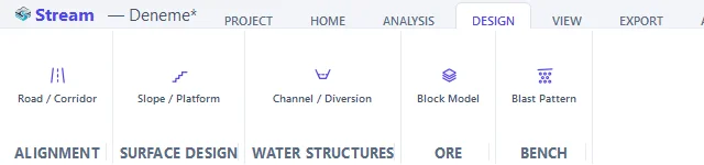
Road / Corridor
Open it from DESIGN ▸ ALIGNMENT ▸ Road / Corridor.
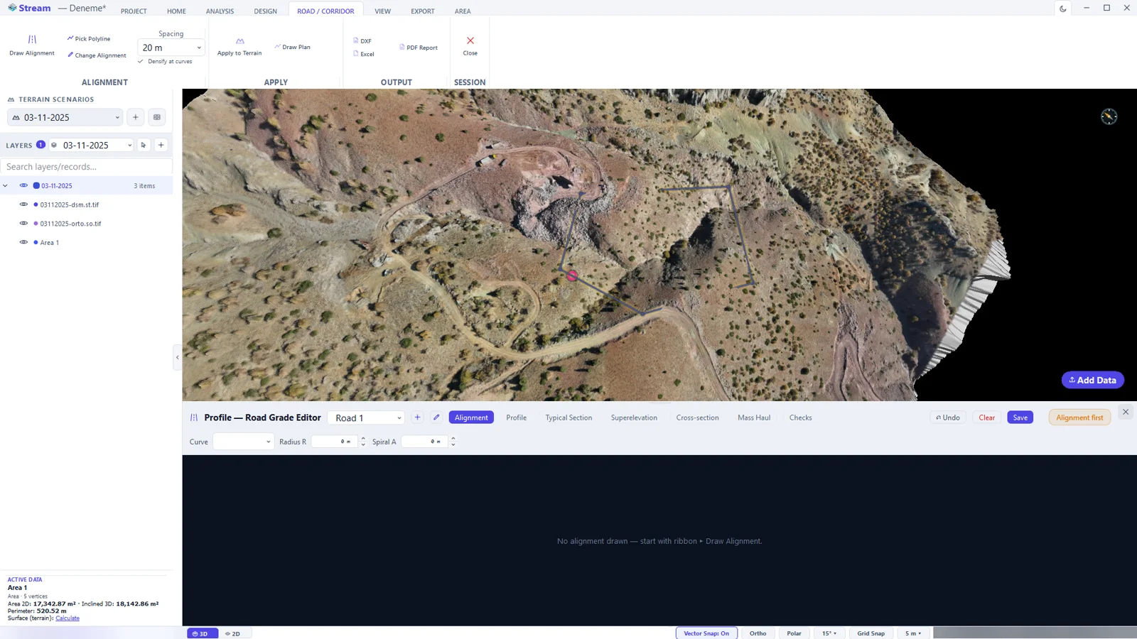
- Alignment — the horizontal axis: PI vertices, curve radius and spiral transitions.
- Profile — the vertical axis: PVI points, grades and vertical curves.
- Typical Section — carriageway width, shoulder and cut/fill batters.
- Superelevation — cross slope through the curves.
- Cross-section — the section at each station with its cut and fill areas.
- Mass Haul — cut/fill balance and haul distance.
- Checks — maximum grade, minimum radius and sight distance are checked on every change.
Plan, profile and cross-sections export to DXF; the quantities to a table; the design report to PDF.
Slope / Platform
Open it from DESIGN ▸ SURFACE DESIGN ▸ Slope / Platform. Draw a closed area, sit it on a flat platform and tie its edges back to the terrain with benched slopes.
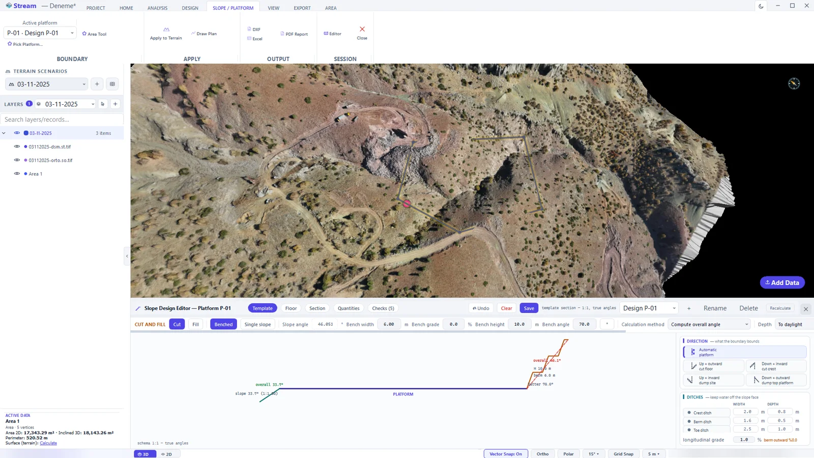
- CUT AND FILL — Benched or Single slope; slope angle, bench width, bench height and bench angle. One of them is derived from the others and its box is locked, so the set always stays consistent.
- DIRECTION — what the boundary is: a cut floor, a cut crest, a dump site or the top platform of a dump.
- DITCHES — crest, berm and toe ditches that keep water off the slope face.
- Floor, Section, Quantities and Checks — the platform level, the section through the design, the cut and fill volumes, and the list of rule violations (overall angle, berm width, a design that never daylights …).
Channel / Diversion
Open it from DESIGN ▸ WATER STRUCTURES ▸ Channel / Diversion. Draw the alignment, or turn an existing line into the channel axis.
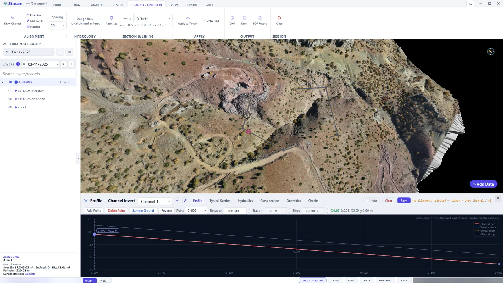
- Profile — the invert: ground elevation, bed elevation and grades.
- Typical Section — bed width, depth, batters and lining.
- Hydraulics — normal depth, velocity, critical depth and Froude number at every station.
- Cross-section, Quantities and Checks — where the channel meets the ground, how much is excavated, and the design review (freeboard, flow regime, permitted velocity …).
Block Model
Open it from DESIGN ▸ ORE ▸ Block Model. The module does not build a block model: it imports the table produced by another package and reads it against the terrain and the pit design.
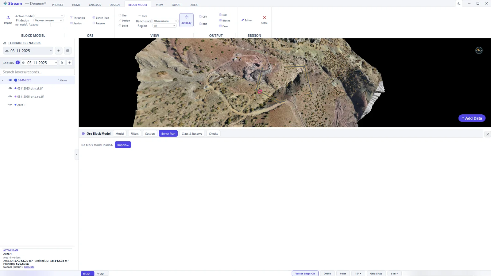
- Import… opens a four-step wizard: file, column mapping, roles and units, validation.
- Model, Filters, Section, Bench Plan, Class & Reserve and Checks — the identity of the model, the grade cut-off, the section through model and pit, tonnage per bench, the resource classes and the validation findings.
Blast Pattern
Open it from DESIGN ▸ BENCH ▸ Blast Pattern. Outline the block on a surveyed bench, draw the face line along the crest and lay out the holes.
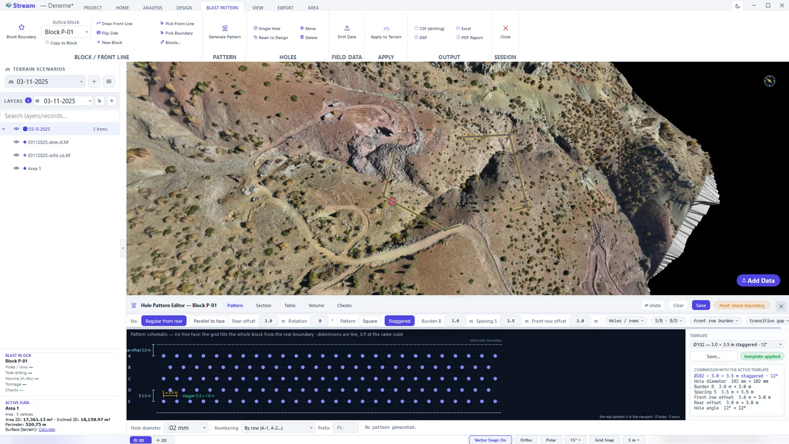
- Pattern — square or staggered layout; burden, spacing, front-row offset and rotation.
- Section, Table, Volume and Checks — the bench section, the hole-by-hole table, the blasted volume and tonnage, and the geometric checks.
- Collar elevations are read from the terrain, so hole depths follow the real bench.
Export and reports
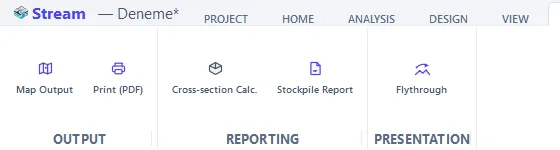
The EXPORT tab writes results out of STREAM.
Map Output
Map Output is the single export gate for data.
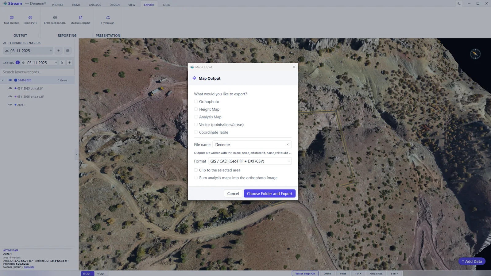
- Click EXPORT ▸ OUTPUT ▸ Map Output.
- Tick what to export: Orthophoto, Height Map, Analysis Map, Vector (points/lines/areas) and Coordinate Table.
- Type a File name and choose the Format: GIS / CAD (GeoTIFF + DXF/CSV), Google Earth (KMZ), LandXML or Shapefile.
- Optionally tick Clip to the selected area and Burn analysis maps into the orthophoto image.
- Press Choose Folder and Export. Every file is written into that one folder.
Print (PDF)
Print (PDF) lays the visible terrain, orthophoto, analysis maps and drawings out on a scaled sheet with a title block.
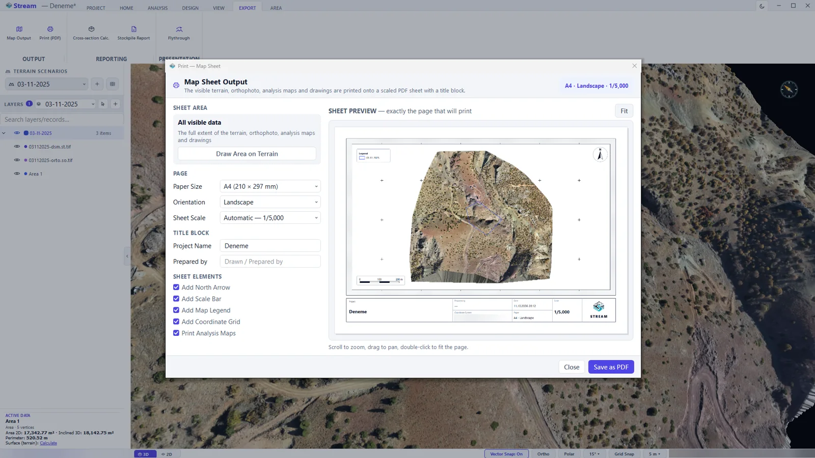
- Click EXPORT ▸ OUTPUT ▸ Print (PDF).
- SHEET AREA — print all visible data, or press Draw Area on Terrain and pick the region with two clicks.
- PAGE — Paper Size (A4 to A0), Orientation and Sheet Scale (automatic picks the largest round scale that fits).
- TITLE BLOCK — Project Name and Prepared by.
- SHEET ELEMENTS — north arrow, scale bar, legend, coordinate grid and analysis maps.
- Check the preview — scroll to zoom, drag to pan — and press Save as PDF.
Reports and presentation
- Cross-section Calc. produces a station-by-station area and volume schedule along an axis, with the cross-section drawing in DXF.
- Stockpile Report collects every stockpile on the site into one PDF: a numbered site view, a summary table and a page per pile.
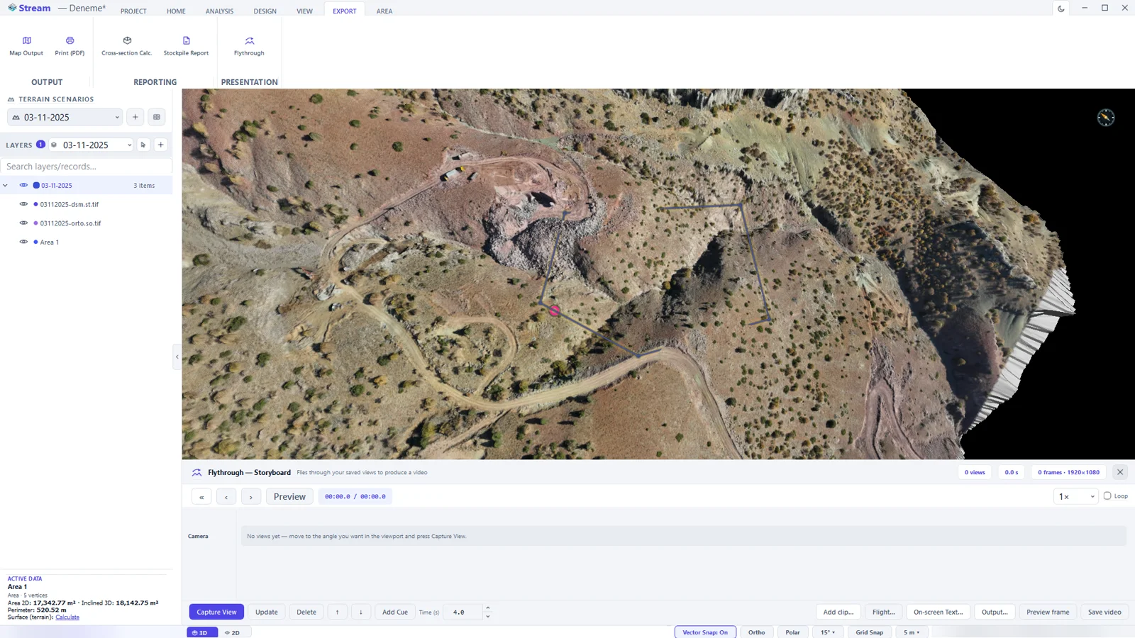
- Flythrough records a camera flight. Move to a view and press Capture View, navigate, capture again; STREAM glides between the views. Preview plays it, Output… sets resolution and frame rate, Save video renders it.
Experimental modules
Permit Audit
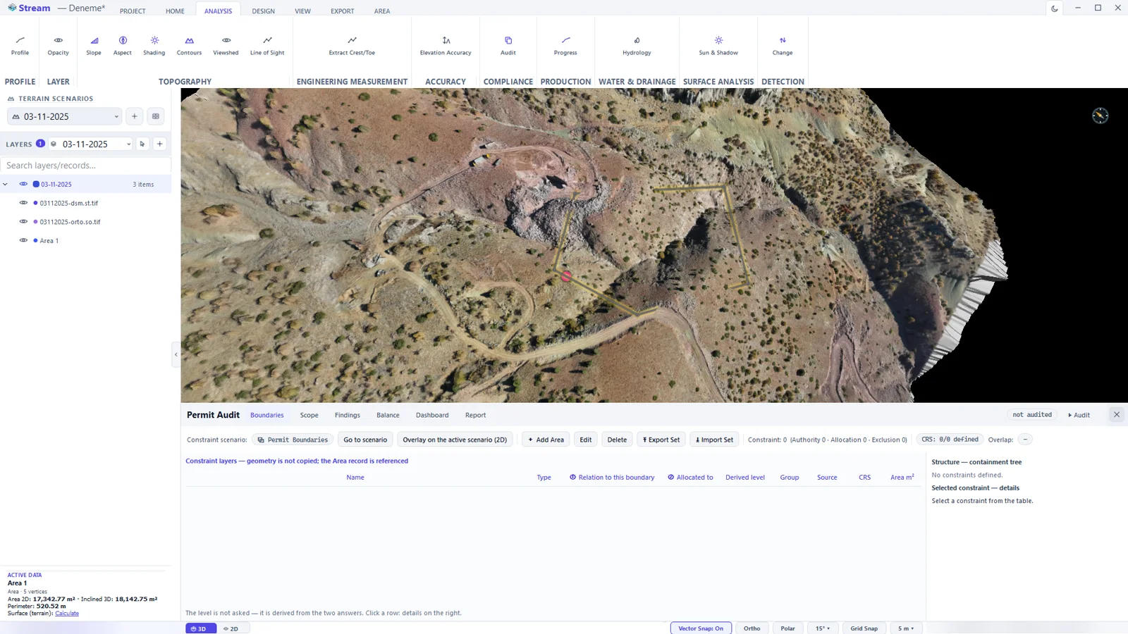
ANALYSIS ▸ COMPLIANCE ▸ Audit checks whether excavation, dumping, stockpile and road activities stay inside licence and permit boundaries. Boundaries are drawn as areas and turned into constraints; ▶ Audit runs the check and lists the findings.
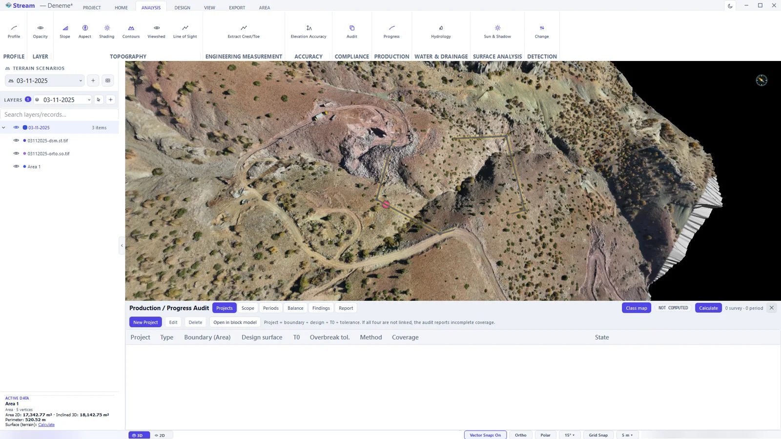
Production / Progress
ANALYSIS ▸ PRODUCTION ▸ Progress classifies the ground movement between dated surveys against the project boundaries and the design level, and produces one report over all periods. A project is a boundary, a design surface, a baseline survey and a tolerance; Calculate runs the audit.
Settings, shortcuts and help
Settings
Open the Home Screen (click the Stream brand) and choose Settings. Changes apply immediately.
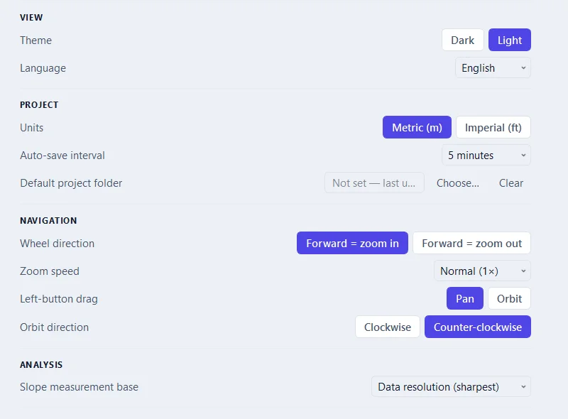
- VIEW — Theme (dark or light) and Language.
- PROJECT — Units (metric or imperial), the Auto-save interval and the Default project folder.
- NAVIGATION — Wheel direction, Zoom speed, what a Left-button drag does (pan or orbit) and the Orbit direction.
- ANALYSIS — the Slope measurement base.
- REPORT — the Prepared by name and the Company Logo printed on PDF reports.
The account and licence cards are at the top of the same page.
Help
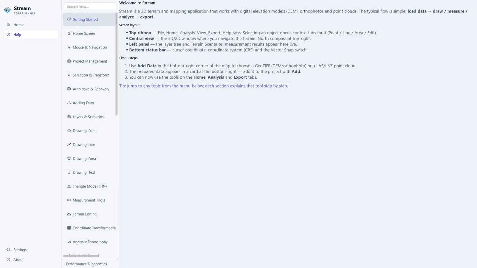
Press F1 at any time: the help opens on the topic of the tool you are using. The Help page of the Home Screen holds the complete guide with a search box.
Keyboard and mouse summary
| Key or action | What it does |
|---|---|
| Left click | Places a point or vertex when a tool is active; selects an object otherwise |
| Right click | Finishes the drawing or measurement |
| Double right click | Leaves the tool |
| Esc | Cancels the drawing in progress |
| Ctrl+Z / Ctrl+Y | Undo / redo |
| Ctrl+N / Ctrl+O / Ctrl+S / Ctrl+Shift+S | New project / open / save / save as |
| L | Load data |
| S | Selection mode (leave the tool) |
| M | Measure distance |
| Ctrl+C / Ctrl+V / Del | Copy / paste / delete the selected object |
| Ctrl+A | Select all |
| Ctrl while selecting | Add to the selection |
| F1 | Help for the active tool |
| Mouse wheel | Zoom toward or away from the cursor |
| Left-button drag | Pan |
| Middle-button drag | Orbit in 3D |
| Arrow keys | Pan · with Shift: rotate and tilt in 3D |
| + / − | Zoom in / out |
| Double-click the compass | Top-down view, north up |
If the terrain feels slow
STREAM draws the terrain on the graphics card and selects the high-performance card by itself at every start. If the terrain is slower than expected, update the graphics driver from the vendor site, plug the laptop in (cards are throttled on battery) and open Help ▸ Performance Diagnostics to see which card is in use.