Volumes and change detection

Cut and fill between two surveys

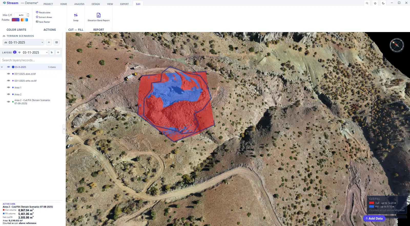
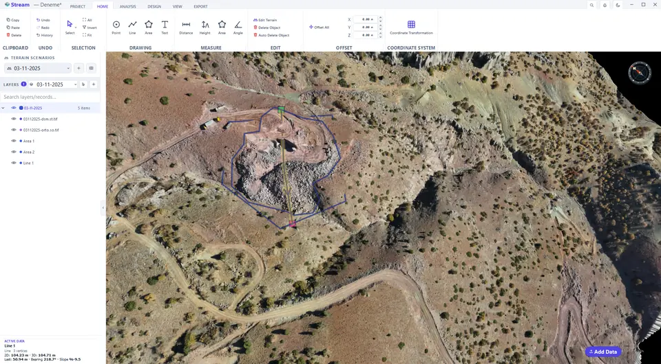
Make the later survey the active scenario, draw an area around the place you want to quantify (HOME ▸ DRAWING ▸ Area) and keep it selected: the AREA tab stays open, and its VOLUMES group holds Cut/Fill, Stockpile and the reference settings. Choose Terrain Scenario as the reference, pick the earlier survey in Scenario and press Cut/Fill. The result is painted inside the area in two colours, and a new record appears in LAYERS, named after the area and the reference.

1. Draw an area, then open Cut/Fill from the Area tab.

   

2. Choose the reference surface.

   

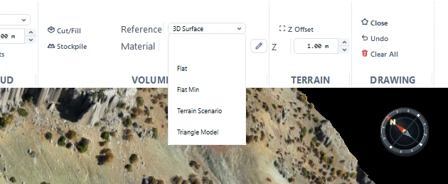
3. Reference set to a terrain scenario.

   

4. Cut and fill result on the terrain.

   

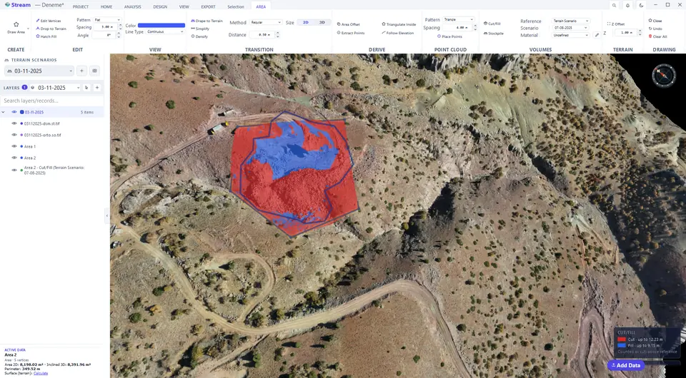
5. Select the result to see its tools.

   

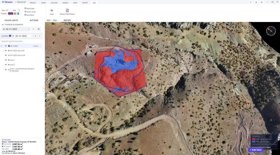
6. Cut and fill volumes in the data card.

   

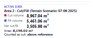
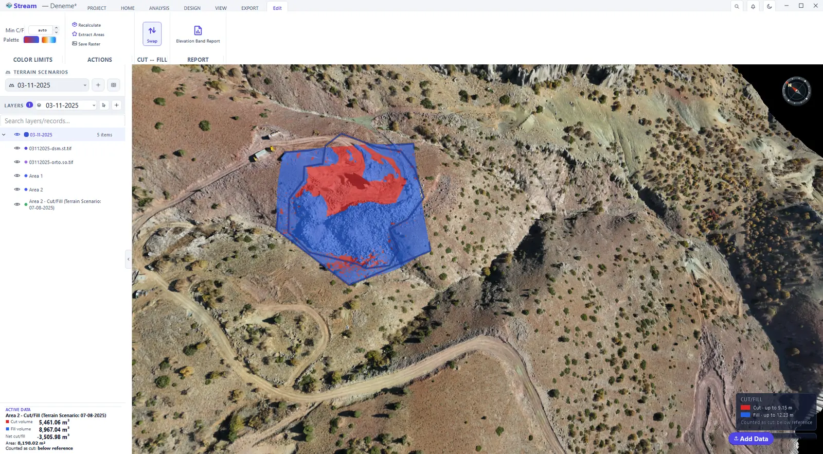
7. Swap the reference direction.

   

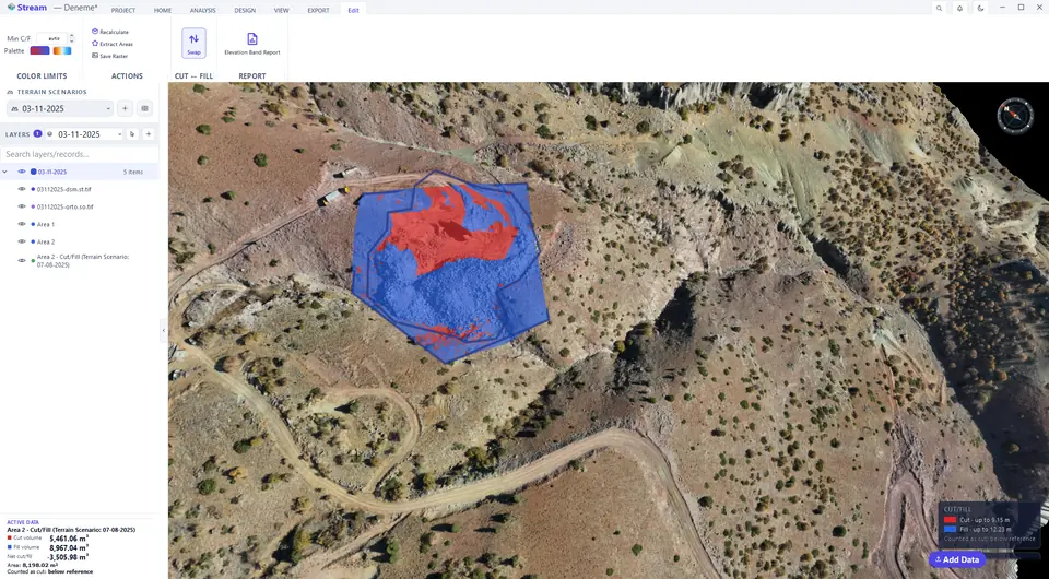
8. Volumes after swapping.

   

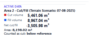
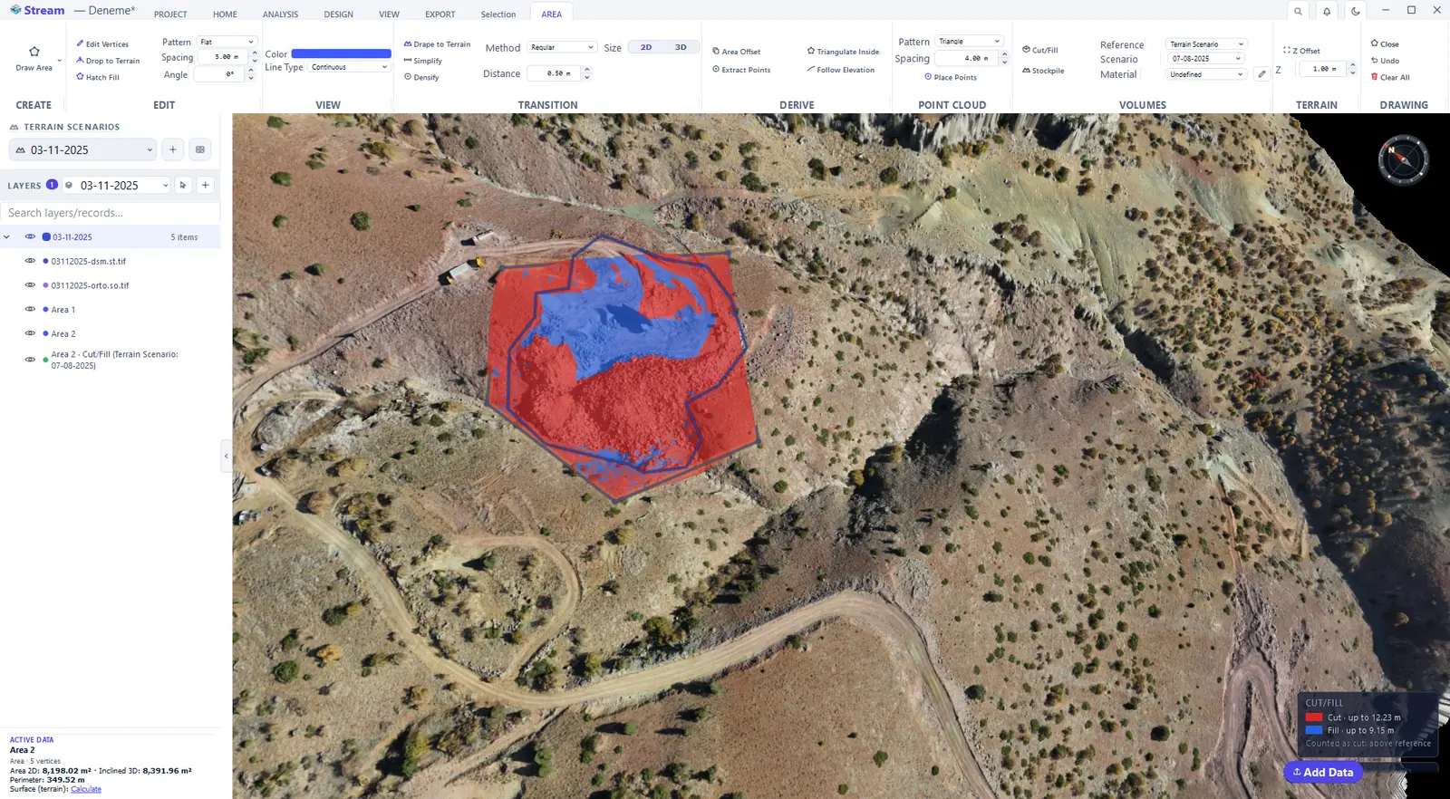
The Reference list decides what the area is compared against:

• 3D Surface — a surface stretched through the corners of the area.
• Flat — a fixed elevation you type.
• Flat Min — a flat base at the lowest corner of the area.
• Terrain Scenario — another survey of the same site.
• Triangle Model — your own design surface (TIN).

Cut (red) is where the active surface lies above the reference; fill (blue) is where it lies below it. The legend at the bottom right of the view names the two colours and gives the deepest cut and the highest fill. Click the map with the Select tool: ACTIVE DATA shows Cut volume, Fill volume, Net cut/fill, the Area and which side is Counted as cut. While a result is still being calculated the card says Calculating… instead of presenting a number as final.

The Edit tab of the map holds the follow-up actions: Recalculate repaints the map with your own colour limits, Extract Areas turns the cut and fill boundaries into editable areas, Save Raster writes the map to a GeoTIFF, Swap exchanges cut and fill and Elevation Band Report splits the volume into bands.

1. Tools of a cut and fill result.

   

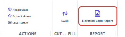
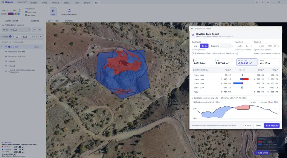
Swap exchanges cut and fill. Use it when the reference is an earlier survey: ground that has been dug away since then is counted — and painted red — as cut, and the heap dumped since then as fill. The volumes, the map colours, the legend and the Elevation Band Report switch together, and the card states which side is counted as cut. Press Swap again to return.

Cut and fill to a flat level

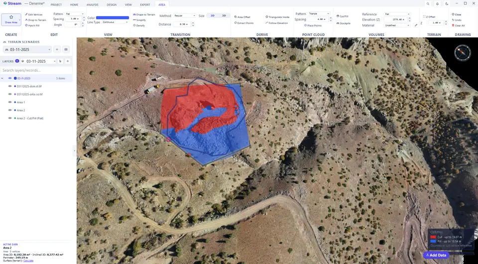
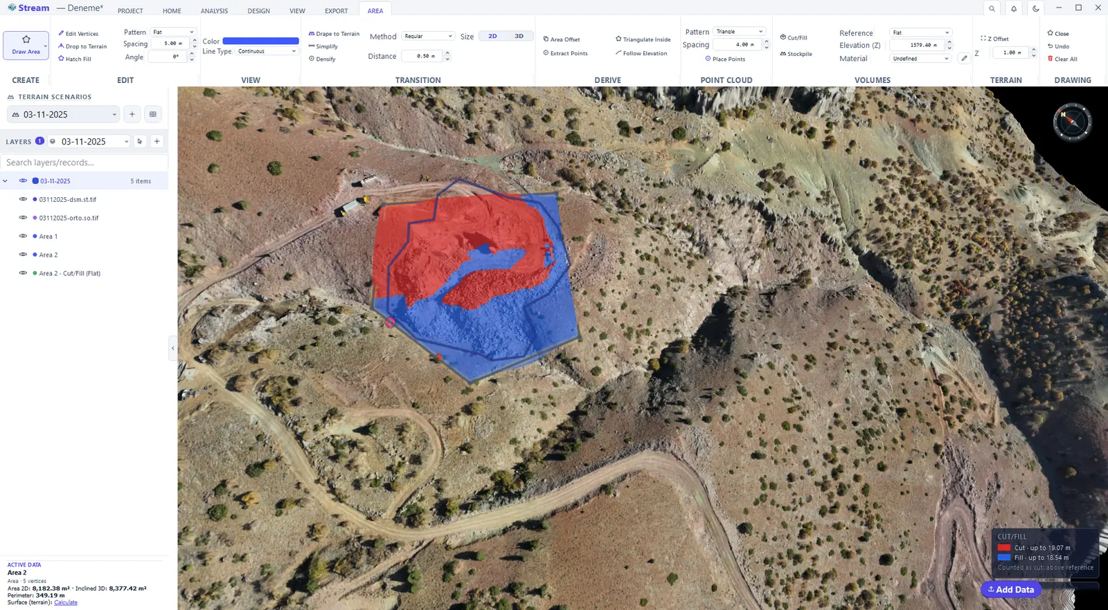
Choose Flat as the reference and type the elevation: the area is compared with a level plane — a pad or a bench floor you plan to build.

1. Choose Flat and type the level.

   

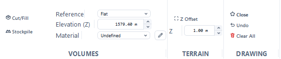
2. Cut and fill against the flat level.

   

Cut and fill to the lowest corner

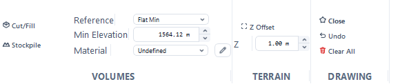
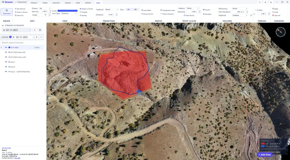
Flat Min uses the lowest corner elevation of the area as a flat base (the minimum elevation is suggested and editable). The cut is then the volume above that level.

1. Flat Min uses the lowest corner of the area.

   

2. Volume above the lowest corner.

   

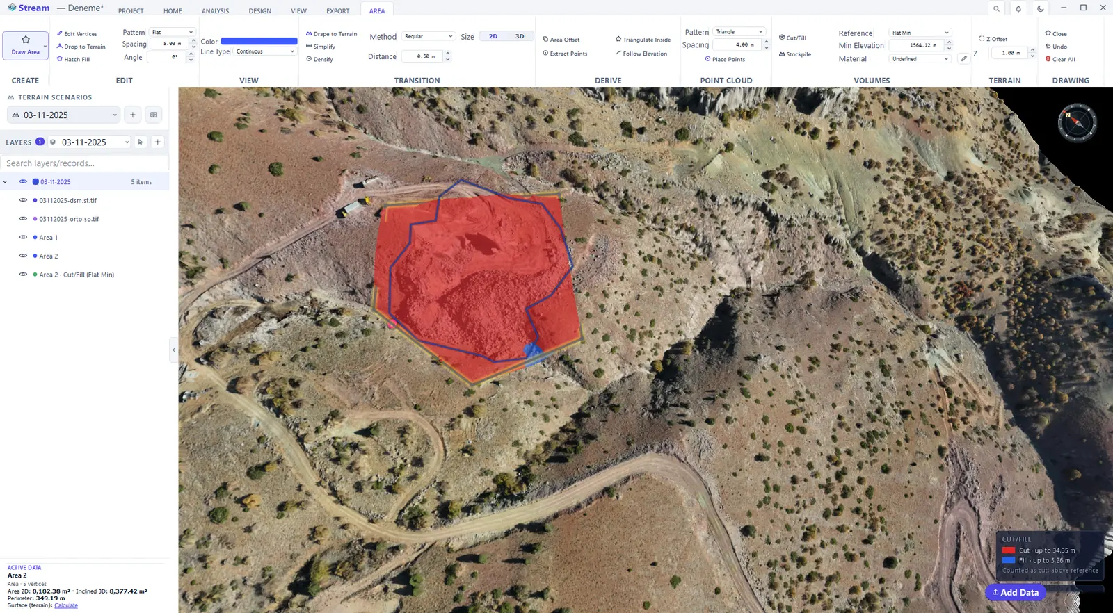
Cut and fill to a 3D surface

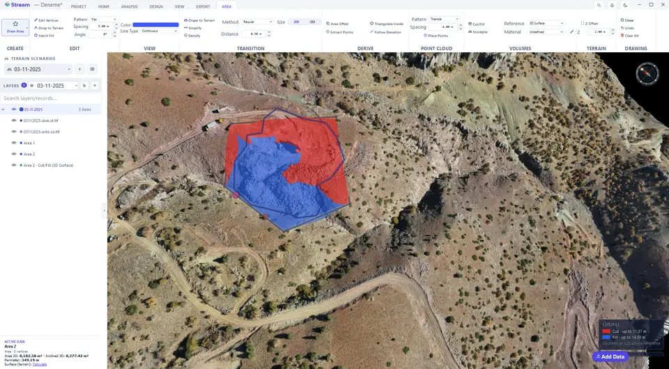
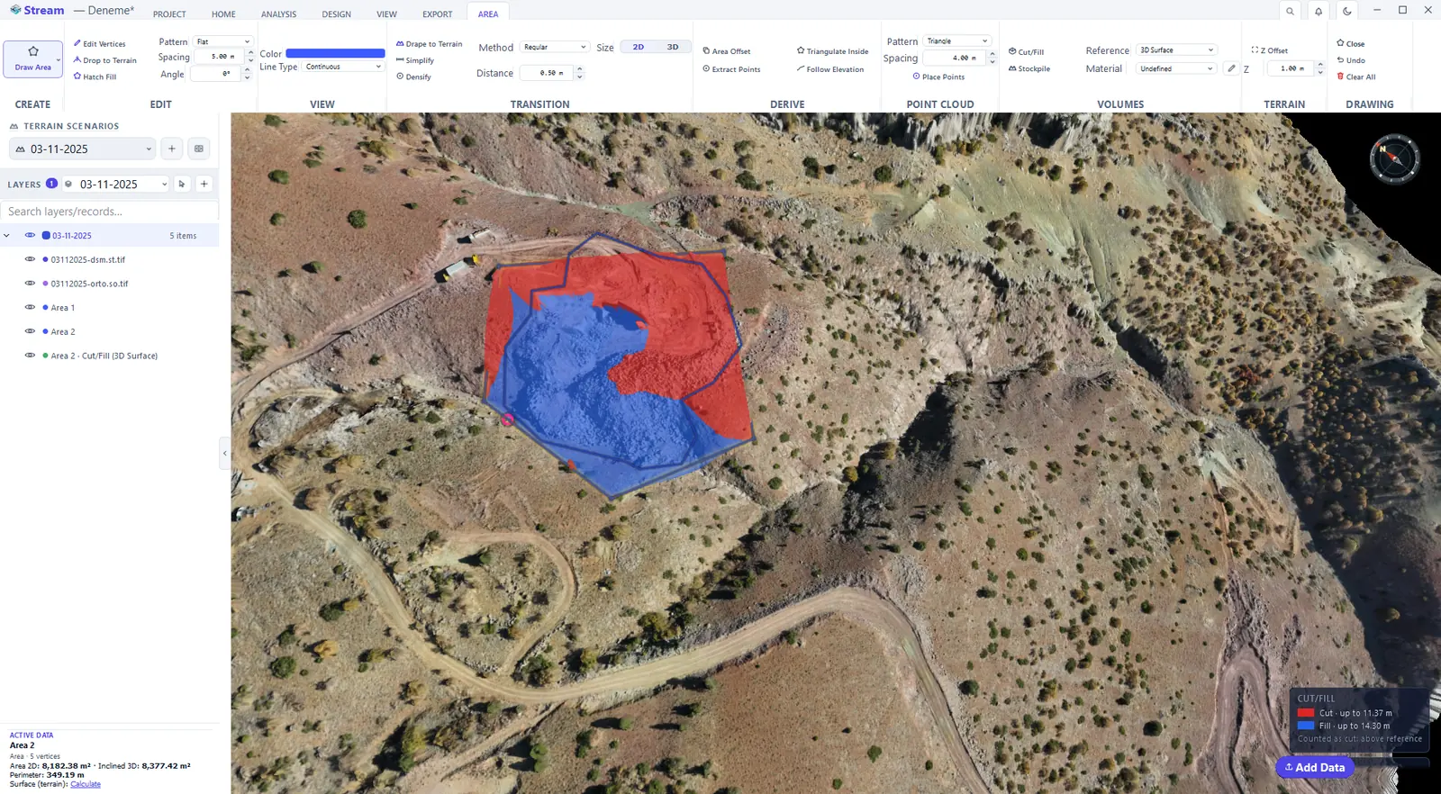
3D Surface stretches a surface through the corners of the boundary. It is the natural base for a pile or a cut that sits on sloping ground.

1. 3D Surface fits a plane through the boundary.

   

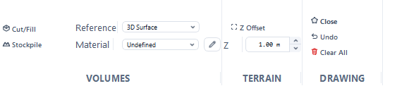
2. Volume against the boundary surface.

   

Elevation band report

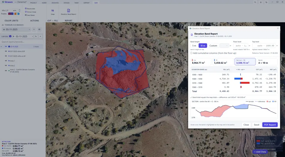
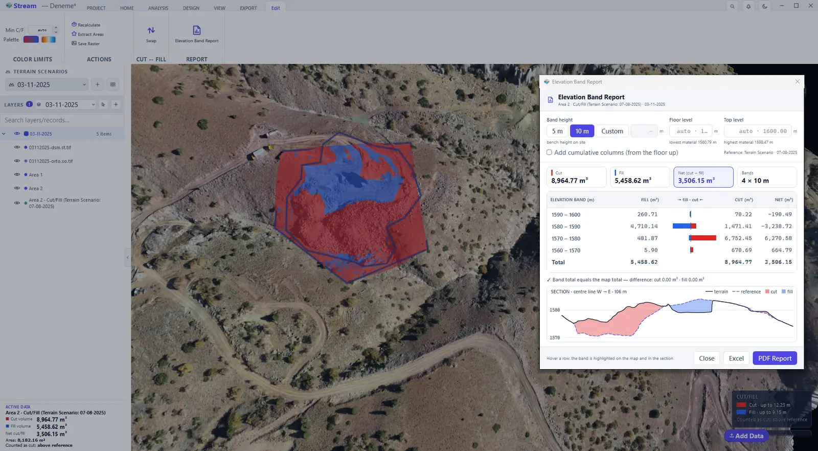
"Floor level 1560, every 10 metres — how much cut and fill is in each band?" The Elevation Band Report answers that from the cut/fill map you already have.

1. Volumes by elevation band.

   

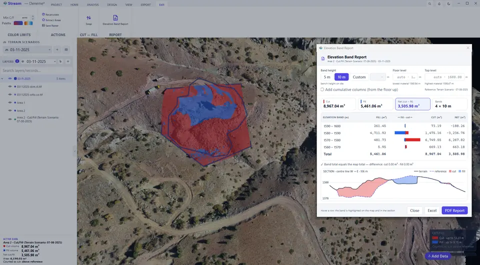
2. Band report after swapping.

   

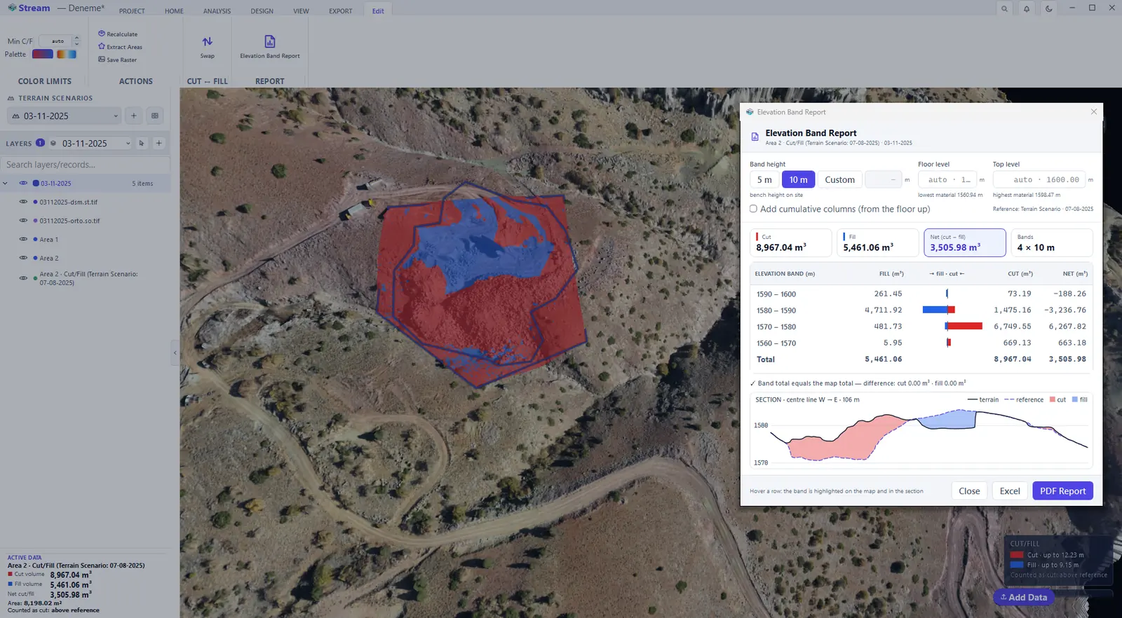
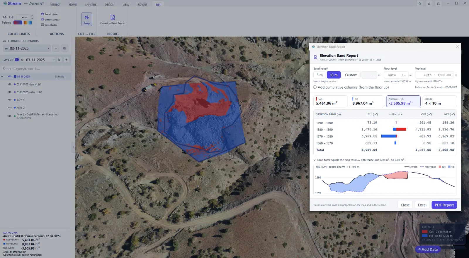
1. Select the cut/fill map and press Elevation Band Report on its Edit tab.
2. Choose the Band height — a preset or Custom. No table is produced until you choose; the bench height of your site is the natural value.
3. Leave Floor level and Top level on auto to cover the whole range where material exists, or type your own levels. Tick Add cumulative columns to sum from the floor up.
4. The row under the table compares the band total with the map total and states the difference. Excel writes the table; PDF Report adds the elevation–volume chart, the site view and the method notes.

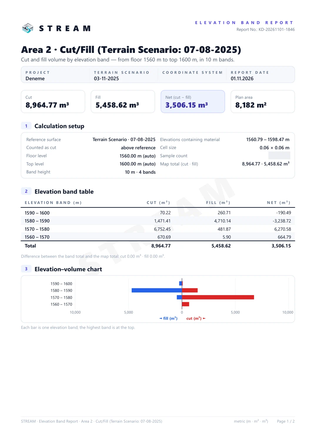
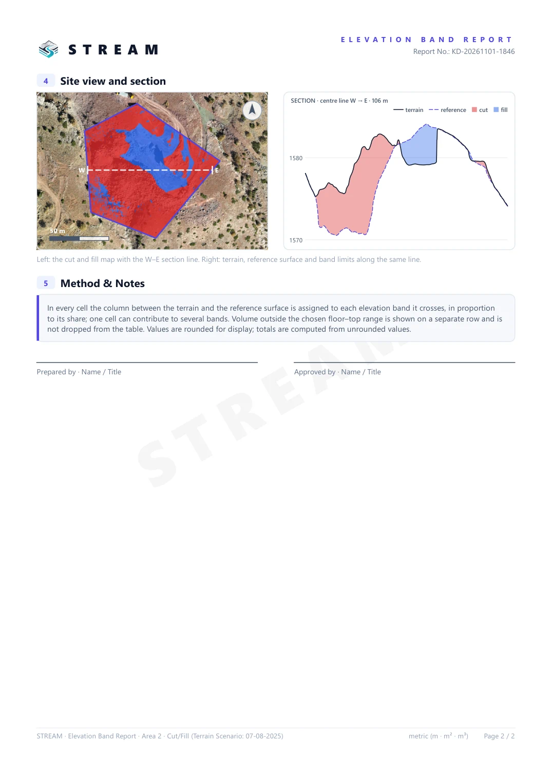
PDF Report writes a two-page document from the numbers on screen — nothing is computed a second time. Page 1 holds the calculation setup (reference surface, which side is counted as cut, floor and top level, band height), the elevation band table and the elevation–volume chart; page 2 shows the cut and fill map with the section line, the section itself and the method notes, with signature lines for Prepared by and Approved by.

1. Elevation Band Report for the cut and fill result.

   

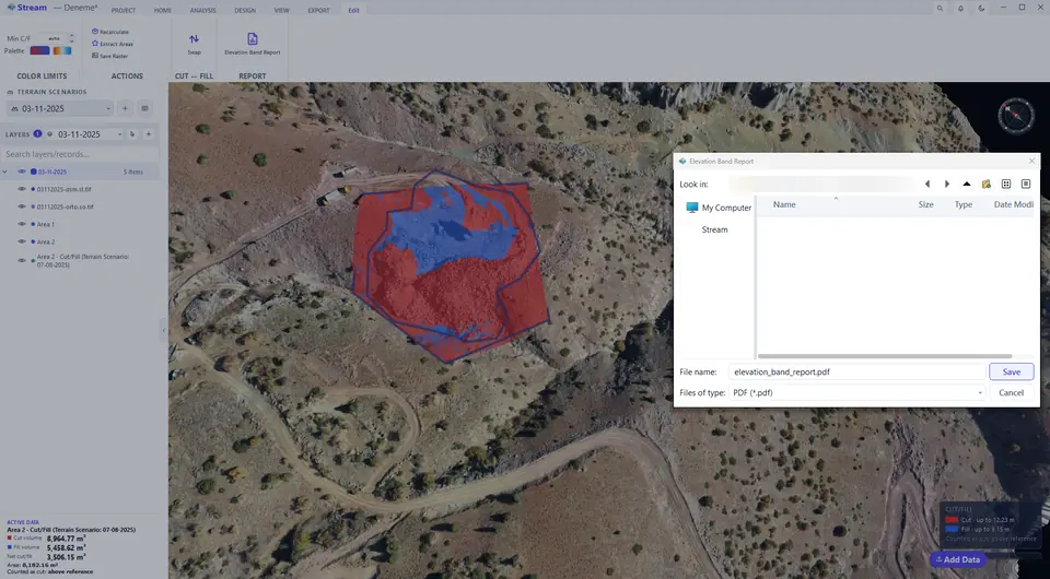
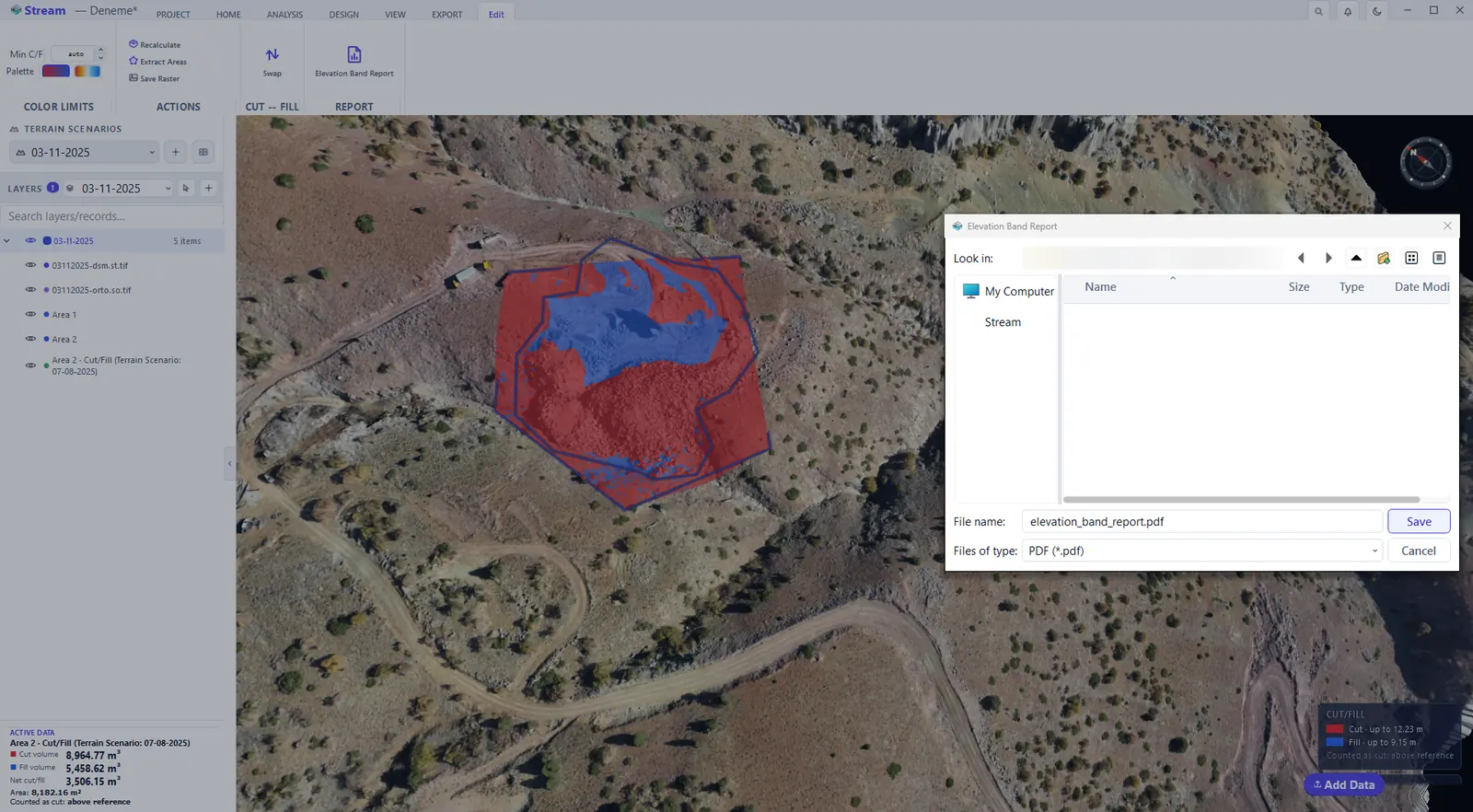
2. Save the report as PDF.

   

3. The finished PDF report, page 1.

   

4. The finished PDF report, page 2.

   

Stockpile volume

A stockpile uses the same volume engine, but the result becomes a pile record with a material attached: density gives tonnage, unit price gives value.

1. Choose Stockpile as the reference.

   

2. Stockpile volume result.

   

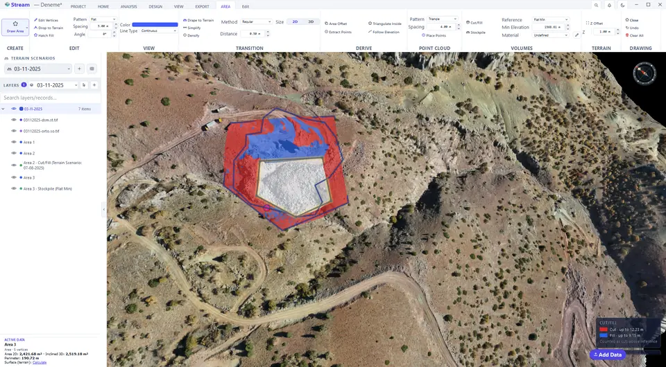
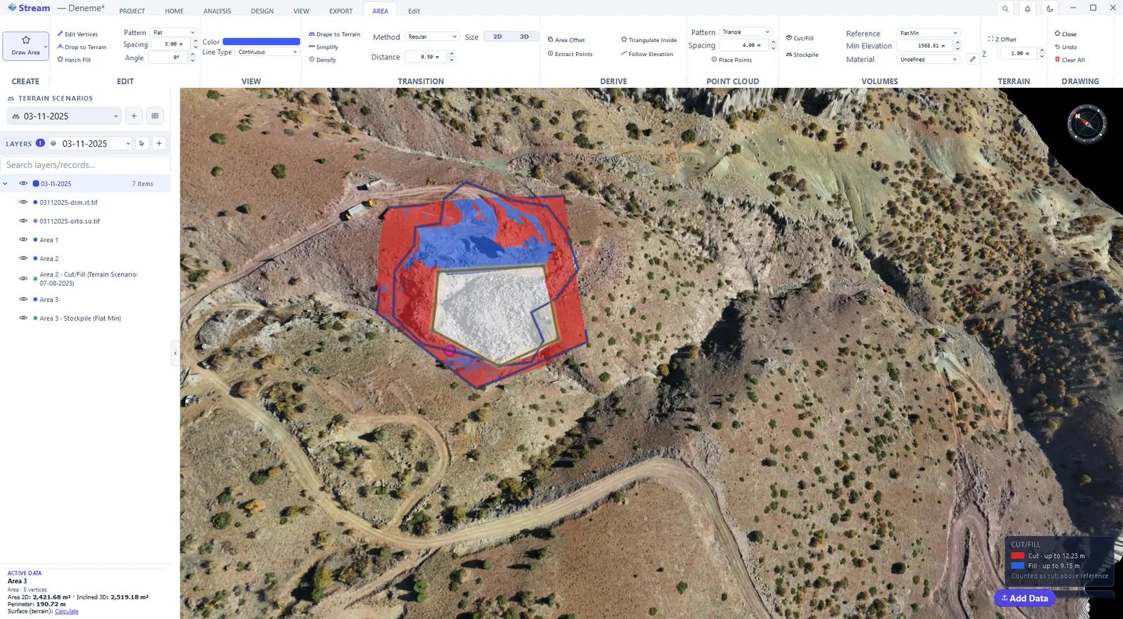
1. Trace the toe of the pile with HOME ▸ DRAWING ▸ Area.
2. On the AREA tab choose the Reference — the base the pile sits on. Flat Min uses the lowest corner; 3D Surface stretches a base through the corners, which suits a pile on sloping ground.
3. Choose the Material (or leave it Undefined — the volume is still correct, only tonnage and value are left out) and press Stockpile.
4. The pile is painted and added to LAYERS. The pencil button next to Material opens the material library: name, colour, density (t/m³) and unit price for each material.
5. EXPORT ▸ REPORTING ▸ Stockpile Report collects every pile on the site into one PDF — see Export and reports.

Cross-section volume

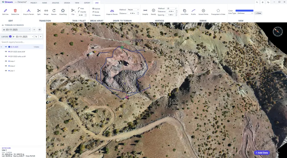
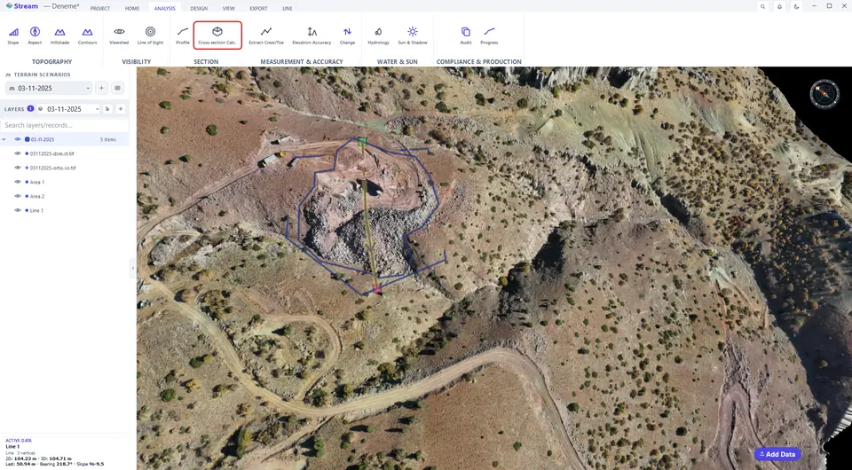
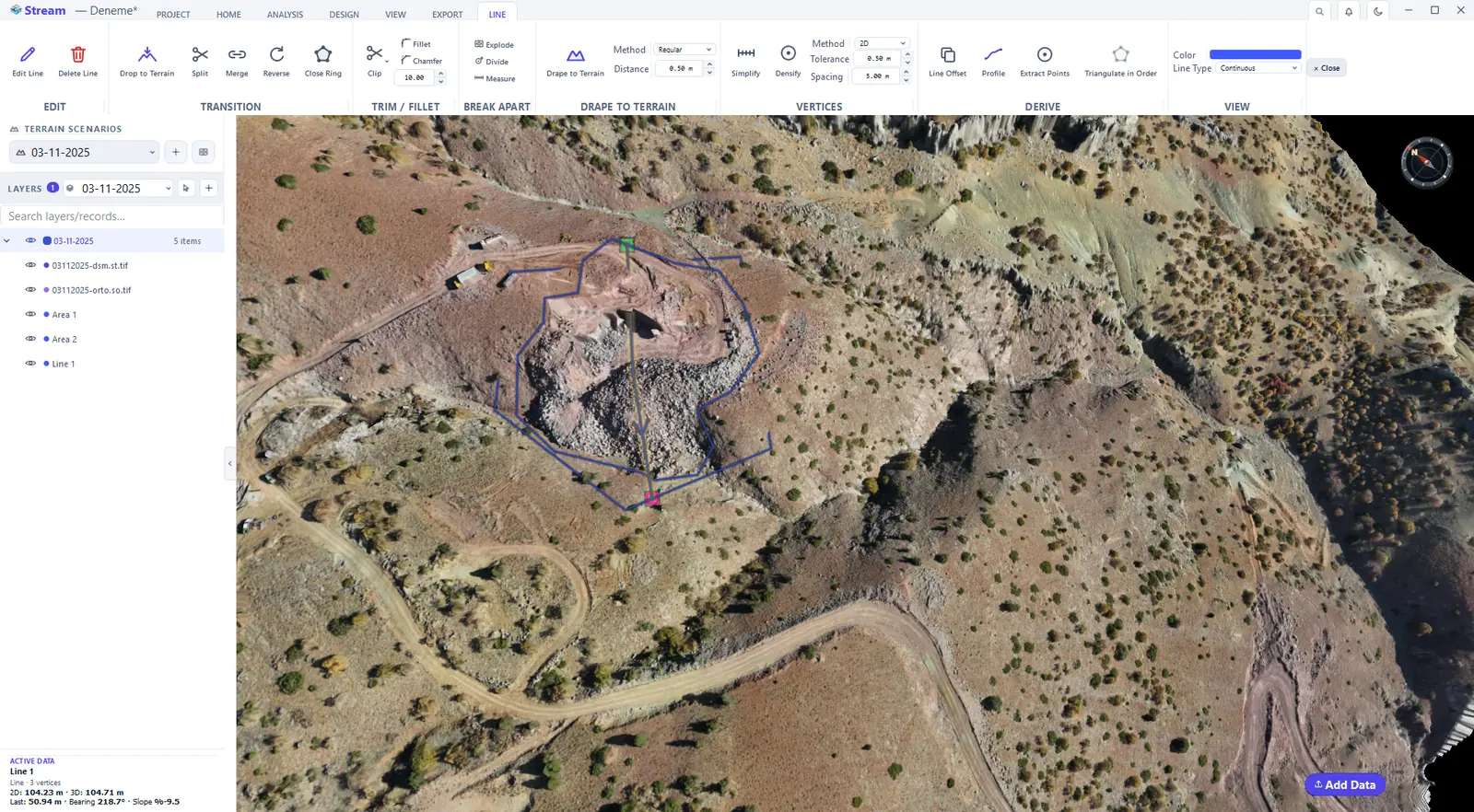
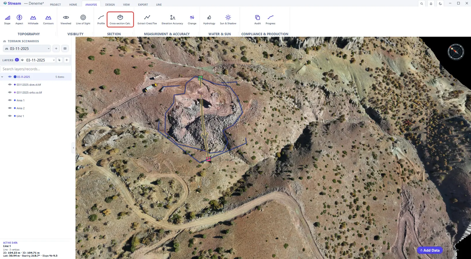
ANALYSIS ▸ SECTION ▸ Cross-section Calc. produces a station-by-station area and volume schedule along an axis, together with the cross-section drawing in DXF. Draw the area that bounds the volume and a centre line across it, then open the tool.

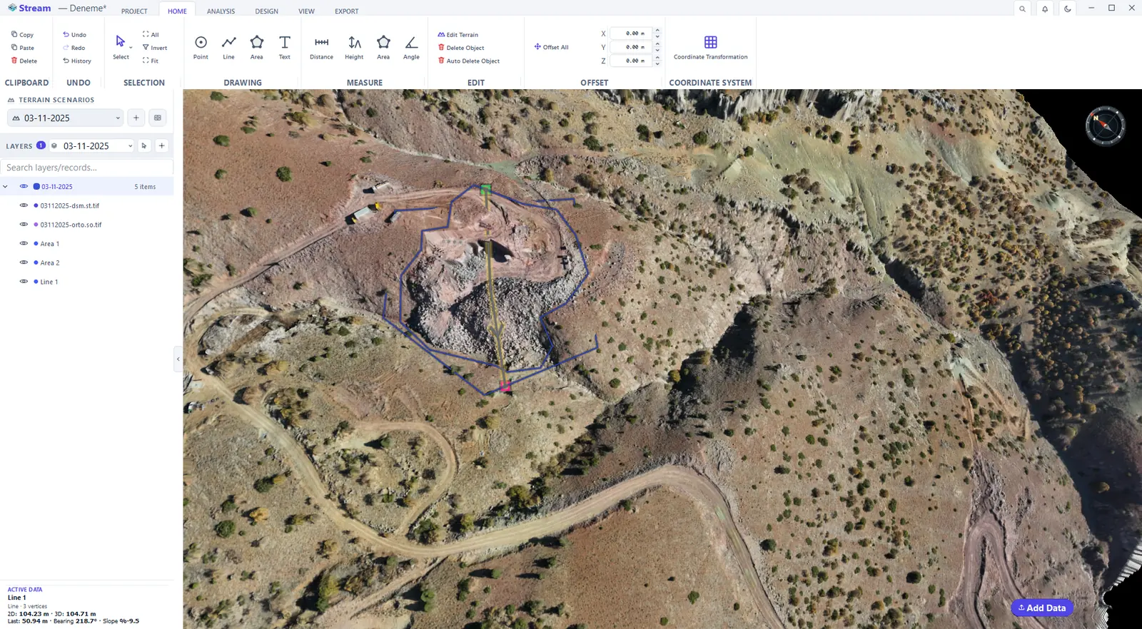
1. Draw an area and a center line across the pit.

   

2. Press Cross-section Volume on the Analysis tab.

   

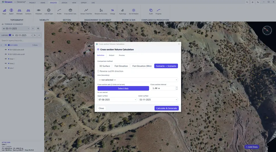
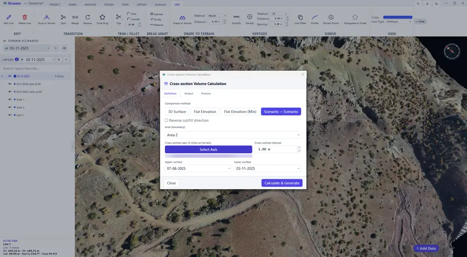
3. Choose the method, boundary, axis, interval and surfaces.

   

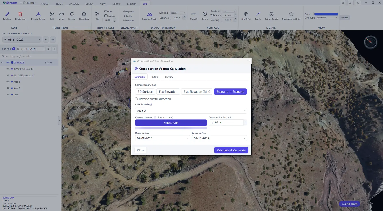
4. Click the center line on the map.

   

5. The axis is set in the dialog.

   

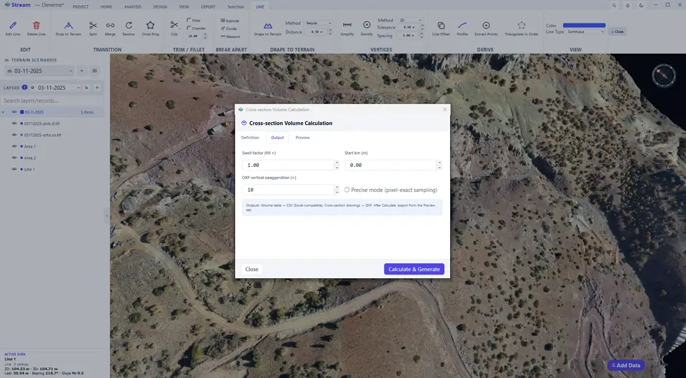
6. Output tab of the section report.

   

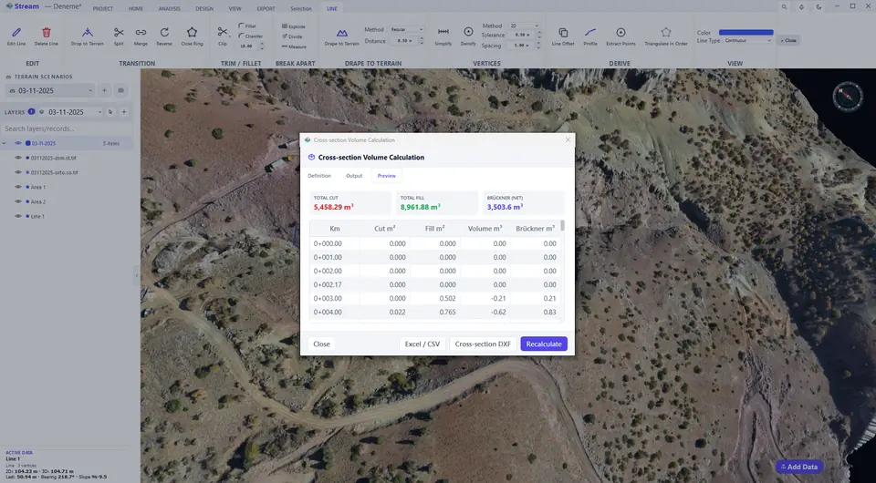
7. Preview tab of the section report.

   

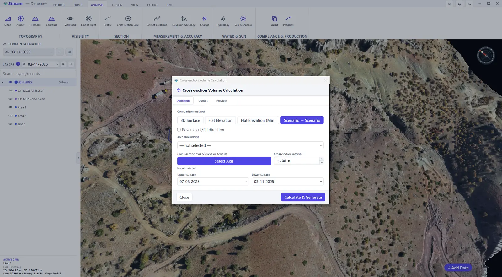
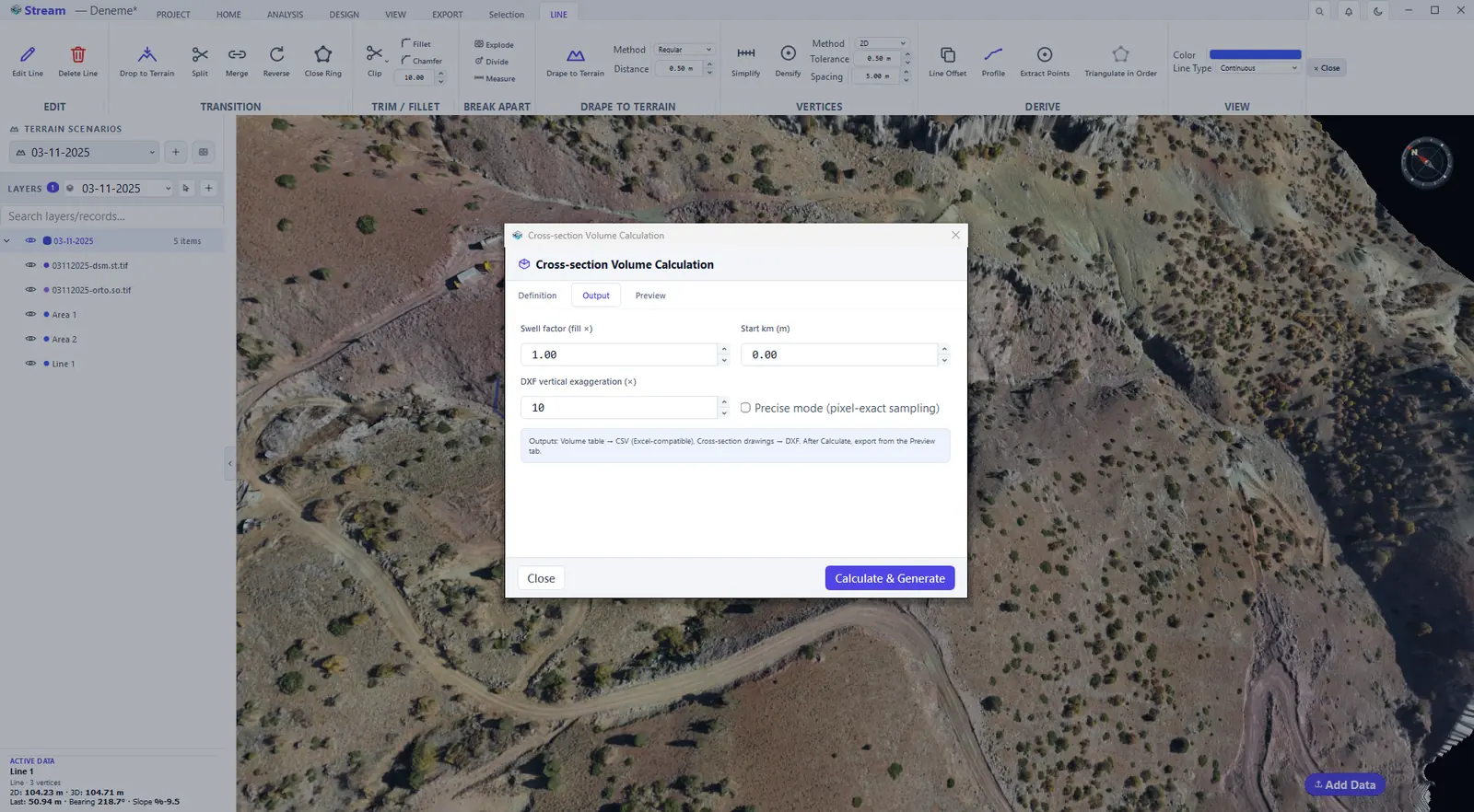
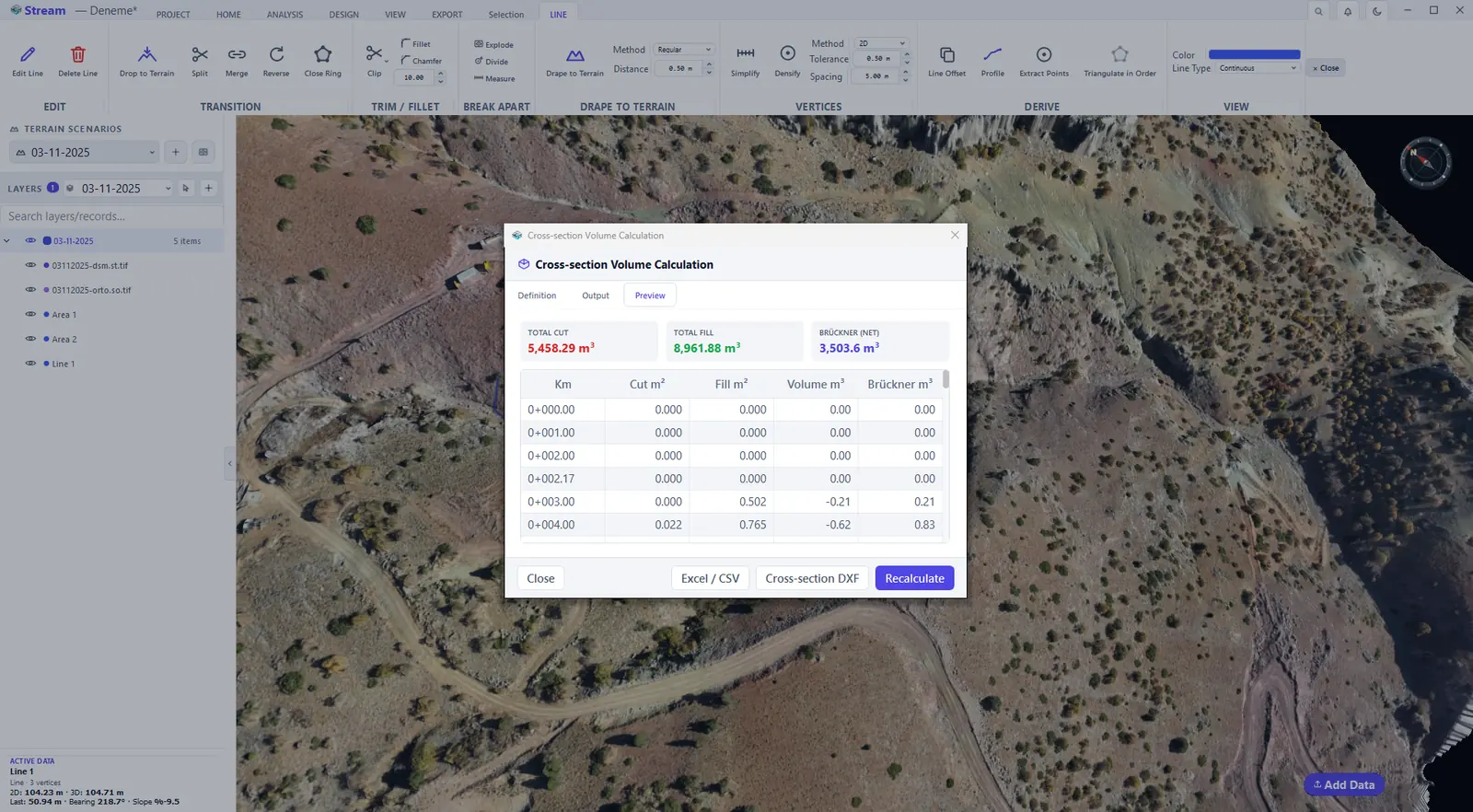
The dialog has three tabs:

• Definition — the comparison method (3D Surface, Flat Elevation, Flat Elevation (Min) or Scenario → Scenario), the Area (boundary), the Cross-section axis (Select Axis, then two clicks on the terrain), the Cross-section interval and the Upper and Lower surface. Reverse cut/fill direction swaps which side counts as cut.
• Output — the Swell factor, the Start km and the DXF vertical exaggeration; tick Precise mode for pixel-exact sampling. The outputs are a volume table (CSV, Excel-compatible) and the cross-section drawings (DXF).
• Preview — after Calculate & Generate, the total cut, the total fill and the net (Brückner) volume, then the station table with the cut area, fill area, volume and Brückner (mass-haul) ordinate at every station. Excel / CSV and Cross-section DXF export the results and Recalculate applies changed settings.

Change detection

Change Detection compares two surveys and separates real change from survey noise. It needs two terrain scenarios and exactly one selected area: make the later survey the active scenario, draw an area around the place you want to check and select it with the Select tool. Then click ANALYSIS ▸ MEASUREMENT & ACCURACY ▸ Change and pick the earlier survey; it becomes the before state.

1. Change Detection button.

   

2. Erosion and deposition map between surveys.

   

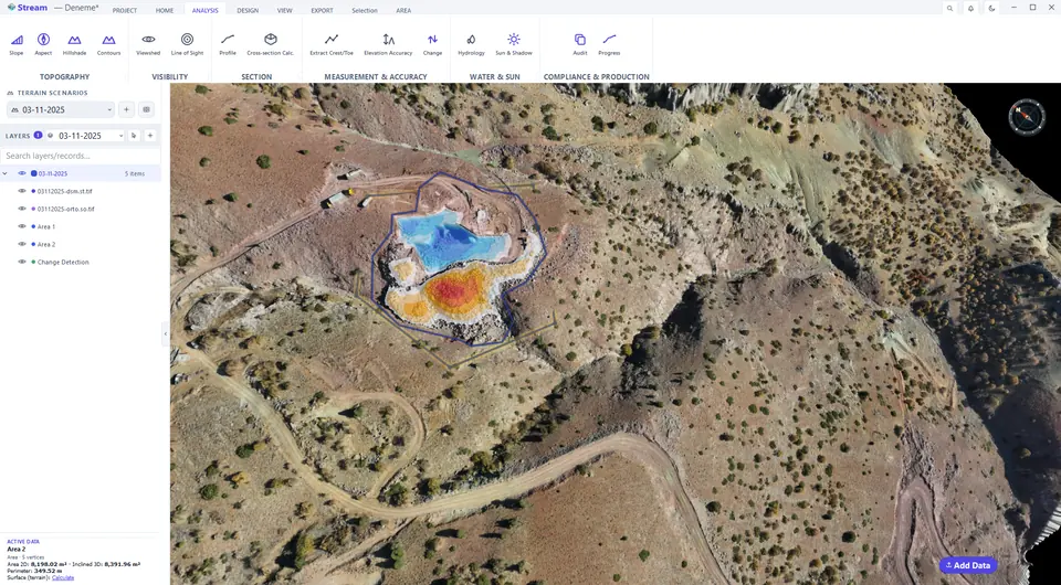
3. Select the result to see its tools.

   

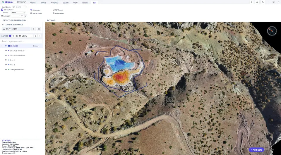
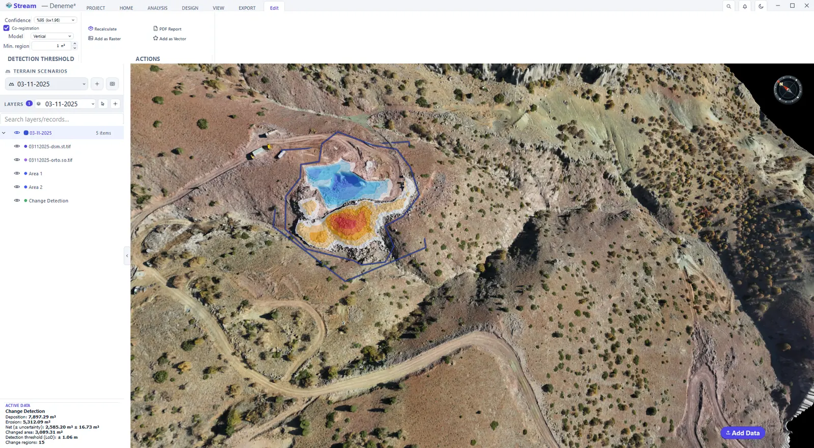
4. Threshold and output controls.

   

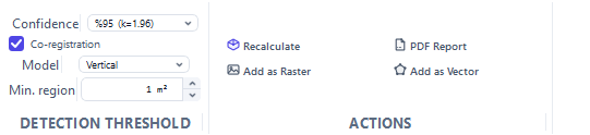
5. Change volumes in the data card.

   

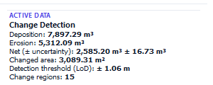
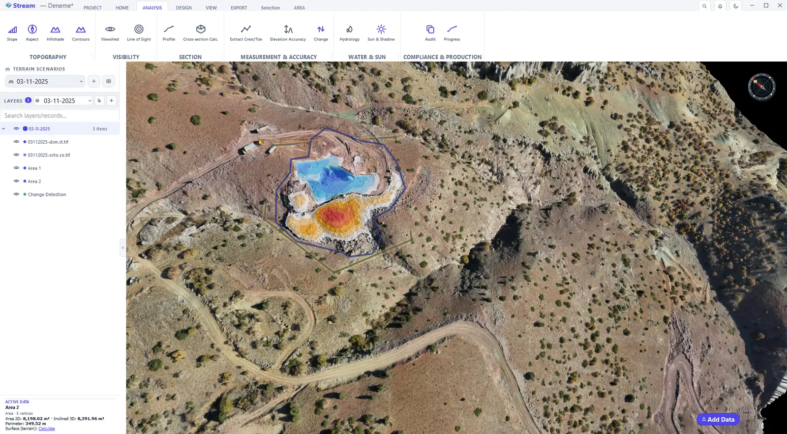
Only the ground that really changed is painted: orange to red where material was removed, blue where it was added. Everything below the detection threshold stays untouched, and a Change Detection record is added to LAYERS. Click the map with the Select tool: ACTIVE DATA reports Deposition, Erosion, the Net volume with its ± uncertainty, the Changed area, the Detection threshold (LoD) and the number of Change regions.

The Edit tab tunes the analysis: Confidence sets the detection threshold — differences smaller than it are treated as survey noise, not change — Co-registration removes a systematic shift between the two surveys before they are compared (Model chooses whether only a vertical shift or also a tilt is removed) and Min. region drops change patches that are too small to be real. Recalculate applies the settings; Add as Raster, Add as Vector and PDF Report keep the result.

Next: Engineering tools.